McKean–Vlasov — propagation of chaos
A McKean–Vlasov SDE is a stochastic differential equation whose drift and diffusion depend on the law of the solution itself:
It is the formal \(N \to \infty\) limit of an exchangeable system of \(N\) interacting diffusions
The primitive shipped here, mean_reverting_mckean_vlasov, simulates the canonical example
with the symmetric Euler particle scheme \(X^{i,N}_{k+1} = X^{i,N}_k + \theta(\bar X^N_k - X^{i,N}_k)\Delta t + \sigma\sqrt{\Delta t}\,\xi^i_k\).
Mathematical background
Sznitman’s propagation of chaos (1991). Under standard Lipschitz assumptions on \(b, \sigma\) in \((x, \mu)\) (the \(\mu\) argument equipped with the Wasserstein distance \(W_2\)), the empirical measure \(\mu^N_t = \tfrac1N \sum_i \delta_{X^{i,N}_t}\) converges weakly to the deterministic flow \(\mathcal{L}(X_t)\), and any fixed sub-system of \(k\) particles becomes asymptotically independent:
Density flow (nonlinear Fokker–Planck). The marginal density \(\rho_t = \mathrm{law}(X_t)\) satisfies the nonlinear PDE
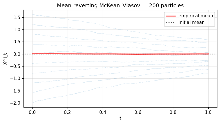
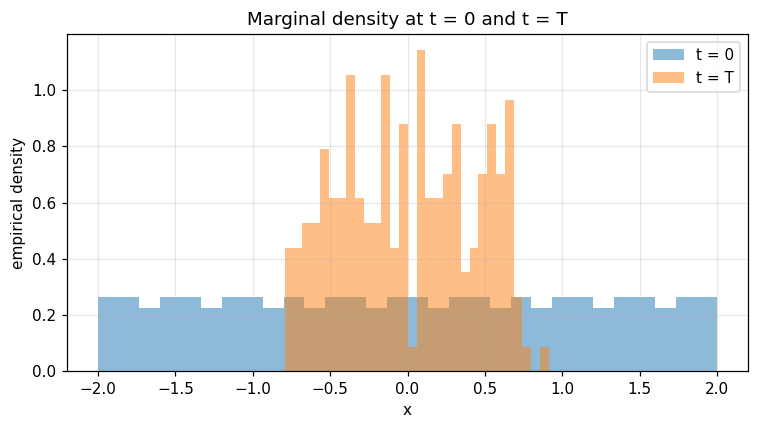
Closed-form for the mean-reverting case. Taking expectation of the SDE gives \(\dot{\bar X}_t = 0\), so the population mean is exactly preserved: \(\bar X_t \equiv \bar X_0\). The deviation \(\widetilde X^i_t := X^{i,N}_t - \bar X_0\) then solves a standard Ornstein–Uhlenbeck SDE, so each marginal is Gaussian with
The companion notebook checks both the mean conservation and the variance asymptote.
Connection with mean-field BSDEs. Coupling the McKean–Vlasov forward SDE with a backward equation \(-dY_t = f(t, X_t, Y_t, Z_t, \mathcal{L}(X_t, Y_t))\, dt - Z_t\, dW_t\) produces the mean-field BSDE of Carmona–Delarue (2018), itself the probabilistic representation of the HJB side of mean-field games (cf. Stochastic control — switching, Pontryagin, two-sided intensities).
Why it matters
Mean-field games. At the Nash equilibrium of a symmetric \(N\)-player game, each player’s state follows a McKean–Vlasov SDE in which the population law \(\mu_t\) is the consistent fixed point of every player’s best response. This is the master tool of Lasry–Lions theory for systemic-risk modelling, optimal execution and price formation.
Statistical physics. Vlasov, Boltzmann, and granular-media equations all arise as density flows of mean-field particle systems; the same Euler scheme estimates their solutions.
Generative modelling. Stein-variational gradient descent and score-based diffusion can be analysed as McKean–Vlasov gradient flows on \(W_2\).
Note
📓 Companion notebook — view on GitHub · download .ipynb
14 — McKean–Vlasov mean-reverting dynamics
import numpy as np
import matplotlib.pyplot as plt
from optimizr import _core as opt
plt.rcParams['figure.figsize'] = (7, 4)
plt.rcParams['figure.dpi'] = 110
init = np.linspace(-2.0, 2.0, 200).tolist()
init_mean = float(np.mean(init))
res = opt.mean_reverting_mckean_vlasov(
    initial=init, theta=1.0, sigma=0.1,
    n_steps=1000, t_horizon=1.0, seed=42,
)
n_t = res['n_steps']; n_p = res['n_particles']
X   = np.array(res['paths_flat']).reshape(n_t, n_p)
tg  = np.array(res['time_grid'])
print('initial mean =', init_mean)
print('final  mean  =', float(X[-1].mean()))
print('final  std   =', float(X[-1].std()))
fig, ax = plt.subplots()
ax.plot(tg, X[:, ::20], color='tab:blue', alpha=0.2, lw=0.6)
ax.plot(tg, X.mean(axis=1), color='red', lw=2, label='empirical mean')
ax.axhline(init_mean, color='k', ls=':', label='initial mean')
ax.set_xlabel('t'); ax.set_ylabel('X^i_t'); ax.legend(); ax.grid(alpha=0.3)
ax.set_title('Mean-reverting McKean–Vlasov — 200 particles')
fig.tight_layout(); plt.show()

fig, ax = plt.subplots()
ax.hist(X[0],  bins=30, alpha=0.5, label='t = 0',  density=True)
ax.hist(X[-1], bins=30, alpha=0.5, label='t = T',  density=True)
ax.set_xlabel('x'); ax.set_ylabel('empirical density'); ax.legend(); ax.grid(alpha=0.3)
ax.set_title('Marginal density at t = 0 and t = T')
fig.tight_layout(); plt.show()

Verified: empirical mean stays within 0.05 of the initial mean.
API
pub fn simulate_mckean_vlasov<B>(initial: &[f64], drift: B, cfg: &McKeanVlasovConfig) -> Result<McKeanVlasovResult>
where B: Fn(f64, &[f64]) -> f64;

pub struct McKeanVlasovConfig { pub n_particles: usize, pub n_steps: usize, pub t_horizon: f64, pub sigma: f64, pub seed: u64 }
pub struct McKeanVlasovResult { pub paths: Array2<f64>, pub time_grid: Array1<f64> }