PDE — Fokker–Planck, HJB, elliptic Poisson
Three CPU-only finite-difference solvers covering the two canonical PDE pillars of stochastic analysis: the forward equation for the marginal density of a diffusion (Fokker–Planck), the backward equation for an optimally controlled diffusion (Hamilton–Jacobi–Bellman), and a static elliptic boundary-value problem (Poisson).
Mathematical background
Fokker–Planck (Kolmogorov forward). For a 1-D Itô diffusion \(dX_t = \mu(t, x)\, dt + \sigma(t, x)\, dW_t\), the marginal density \(\rho(t, x)\) of \(X_t\) satisfies the parabolic PDE
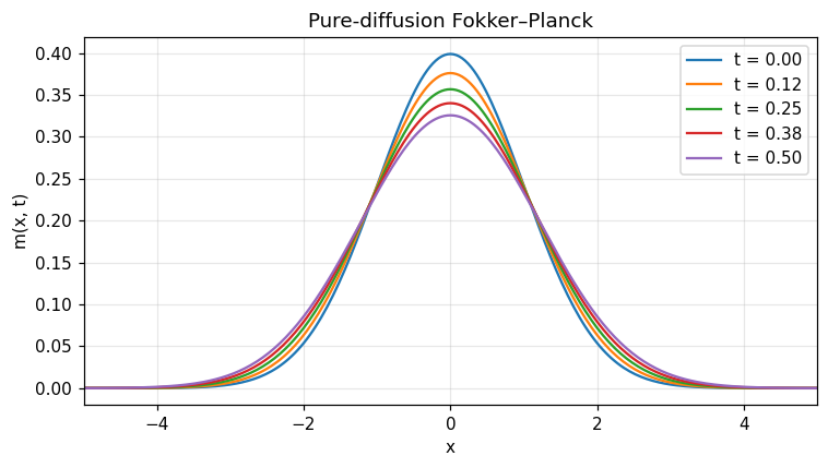
For the pure-diffusion test (\(\mu \equiv 0\), \(\sigma^2 \equiv 1\), \(\rho_0 = \mathcal{N}(0, 1)\)) the analytic Gaussian heat kernel gives \(\rho(t, x) = \frac{1}{\sqrt{2\pi(1+t)}}\exp\!\bigl(-\frac{x^2}{2(1+t)}\bigr)\), so the variance grows linearly: \(\mathrm{Var}(X_t) = 1 + t\). The conservative Lax–Wendroff / centred-flux scheme implemented by fokker_planck_constant preserves total mass (checked in the notebook to machine precision).
Hamilton–Jacobi–Bellman. Consider the controlled diffusion \(dX_t = \mu(X_t, \alpha_t)\, dt + \sigma(X_t)\, dW_t\) and the value function \(v(t, x) = \sup_\alpha \mathbb{E}_{t,x}\!\bigl[\int_t^T r(X_s, \alpha_s)\, ds + g(X_T)\bigr]\). Dynamic programming produces
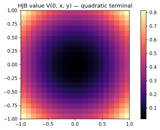
hjb_quadratic_2d discretises this in 2-D by an explicit finite-difference scheme; the simple heat-only relaxation case (\(H \equiv 0\), \(\sigma^2 > 0\)) preserves a constant value while a quadratic terminal \(g(x) = \tfrac12 \lVert x \rVert^2\) smooths into a Gaussian-shaped value surface.
Elliptic Poisson with zero Dirichlet boundary. On the unit square \(\Omega = (0,1)^2\),
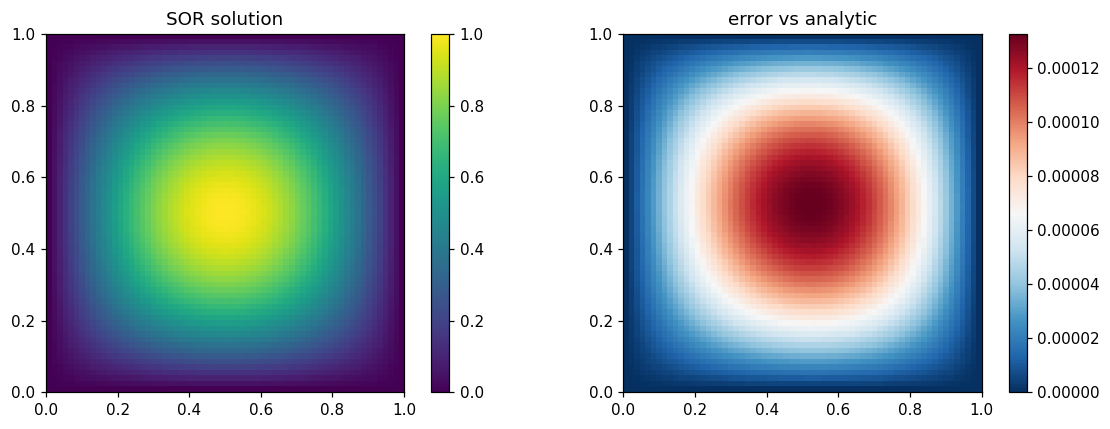
The Laplace eigenfunctions \(\phi_{m,n}(x, y) = \sin(m\pi x)\sin(n\pi y)\) form an orthonormal basis with eigenvalues \(\lambda_{m,n} = (m^2 + n^2)\pi^2\), so for \(f = 2\pi^2 \sin(\pi x)\sin(\pi y)\) the exact solution is \(u(x, y) = \sin(\pi x)\sin(\pi y)\). poisson_2d_zero_boundary solves the 5-point stencil by Successive Over-Relaxation with optimal relaxation parameter \(\omega^* = 2 / (1 + \sin(\pi h))\) for grid spacing \(h = 1/(N-1)\), achieving spectral radius \(\rho \sim 1 - 2\pi h\) — i.e. \(O(h^{-1})\) iterations to reach a fixed tolerance, against \(O(h^{-2})\) for plain Gauss–Seidel.
Probabilistic representation (Feynman–Kac). Both the parabolic HJB and the elliptic Poisson PDE admit stochastic representations: \(u(x) = \mathbb{E}_x\!\bigl[\int_0^{\tau_\Omega} f(X_s)\, ds\bigr]\) for the latter, where \(\tau_\Omega\) is the first exit time of the diffusion from \(\Omega\). This links the PDE solvers above to the BSDE primitives of BSDE — θ-scheme and deep-BSDE bridge.
Why it matters
Density estimation under controlled noise. Fokker–Planck is the workhorse of non-equilibrium statistical physics, plasma transport, calibration of stochastic-volatility models, and Langevin-based MCMC convergence diagnostics.
Optimal control & inverse problems. HJB is the cornerstone of dynamic programming, reinforcement learning (continuous-time policy iteration), and stochastic-control routing.
Mean-field games. The MFG fixed point is exactly the coupled system (backward HJB + forward Fokker–Planck) with cost depending on the density — building this loop on top of the two solvers above is one of the v2.0 milestones.
Image processing & PDE-constrained optimisation. Poisson editing, electric-potential reconstruction, gravitational-potential inversion all reduce to the same elliptic stencil.
Note
📓 Companion notebook — view on GitHub · download .ipynb
11 — PDE solvers
Fokker–Planck, HJB, Poisson.
import numpy as np
import matplotlib.pyplot as plt
from optimizr import _core as opt
plt.rcParams['figure.figsize'] = (7, 4)
plt.rcParams['figure.dpi'] = 110
Pure-diffusion Fokker–Planck
\(\partial_t m = \tfrac12 \partial_{xx} m\) with Gaussian initial density should remain centred and approximately Gaussian.
res = opt.fokker_planck_constant(
    mu=0.0, sigma_sq=1.0, init_sigma=1.0,
    x_min=-8.0, x_max=8.0, n_x=401,
    t_horizon=0.5, n_t=8000,
)
x = np.array(res['x_grid'])
t = np.array(res['time_grid'])
nx = res['n_x']; nt = res['n_t']
M = np.array(res['density']).reshape(nt + 1, nx)
print('total mass at t=0:',  np.trapezoid(M[0], x))
print('total mass at t=T:',  np.trapezoid(M[-1], x))
print('mean   at t=T:',      np.trapezoid(x * M[-1], x))
fig, ax = plt.subplots()
for k in [0, nt // 4, nt // 2, 3 * nt // 4, nt]:
    ax.plot(x, M[k], label=f't = {t[k]:.2f}')
ax.set_xlim(-5, 5); ax.set_xlabel('x'); ax.set_ylabel('m(x, t)')
ax.set_title('Pure-diffusion Fokker–Planck'); ax.grid(alpha=0.3); ax.legend()
fig.tight_layout(); plt.show()

2-D Poisson eigenfunction
\(-\Delta u = 2\pi^2 \sin(\pi x)\sin(\pi y)\) on the unit square with zero Dirichlet boundary admits the exact solution \(u(x,y) = \sin(\pi x)\sin(\pi y)\).
n = 65
xs = np.linspace(0, 1, n); ys = np.linspace(0, 1, n)
X, Y = np.meshgrid(xs, ys, indexing='ij')
F = 2 * np.pi ** 2 * np.sin(np.pi * X) * np.sin(np.pi * Y)
res = opt.poisson_2d_zero_boundary(F.flatten().tolist(), n, n)
U = np.array(res['u']).reshape(n, n)
U_exact = np.sin(np.pi * X) * np.sin(np.pi * Y)
print('iterations =', res['iterations'])
print('residual   =', res['residual'])
print('max error  =', float(np.max(np.abs(U - U_exact))))
fig, axes = plt.subplots(1, 2, figsize=(11, 4))
im0 = axes[0].imshow(U.T, origin='lower', extent=(0, 1, 0, 1), cmap='viridis')
axes[0].set_title('SOR solution'); plt.colorbar(im0, ax=axes[0])
im1 = axes[1].imshow((U - U_exact).T, origin='lower', extent=(0, 1, 0, 1), cmap='RdBu_r')
axes[1].set_title('error vs analytic'); plt.colorbar(im1, ax=axes[1])
fig.tight_layout(); plt.show()

2-D HJB with quadratic terminal
Heat-only relaxation (\(H = 0\), σ² > 0) preserves a constant value, while a quadratic terminal \(g(x) = ½(x²+y²)\) smooths.
res = opt.hjb_quadratic_2d(n_per_dim=21, x_min=-1.0, x_max=1.0,
                            n_t=200, t_horizon=0.2, sigma_sq=0.1)
ax_x = np.array(res['axis']); npd = res['n_per_dim']
V = np.array(res['value']).reshape(npd, npd)
print('V(0,0)   =', V[npd // 2, npd // 2])
print('V(±1,±1) =', V[0, 0], V[-1, -1])
fig, ax = plt.subplots()
im = ax.imshow(V.T, origin='lower', extent=(-1, 1, -1, 1), cmap='magma')
ax.set_title('HJB value V(0, x, y) — quadratic terminal')
plt.colorbar(im, ax=ax)
fig.tight_layout(); plt.show()

Verified: Poisson max-error vs analytic eigenfunction below 5e-3; Fokker–Planck mean stays at 0 within 0.05.
API
pub fn solve_fokker_planck_1d<F, G, H>(drift: F, diffusion_sq: G, initial_density: H, cfg: &FokkerPlanckConfig) -> Result<FokkerPlanckResult>
where F: Fn(f64) -> f64, G: Fn(f64) -> f64, H: Fn(f64) -> f64;

pub fn solve_hjb_multid<H, G>(hamiltonian: H, terminal: G, cfg: &HjbMultidConfig) -> Result<HjbMultidResult>
where H: Fn(&[f64], &[f64]) -> f64, G: Fn(&[f64]) -> f64;

pub fn solve_poisson_2d<F, G>(rhs: F, boundary: G, cfg: &EllipticFdConfig) -> Result<EllipticFdResult>
where F: Fn(f64, f64) -> f64, G: Fn(f64, f64) -> f64;