Agent-based — bounded-confidence consensus
Generic symmetric interacting-agent simulator implementing the linear bounded-confidence update rule
with \(\alpha \in (0, 1]\) the averaging weight and \(\sigma\) the noise scale. This is the DeGroot–Friedkin–Johnsen baseline of opinion dynamics, and the complete-graph limit of the Hegselmann–Krause and Vicsek flocking models.
Mathematical background
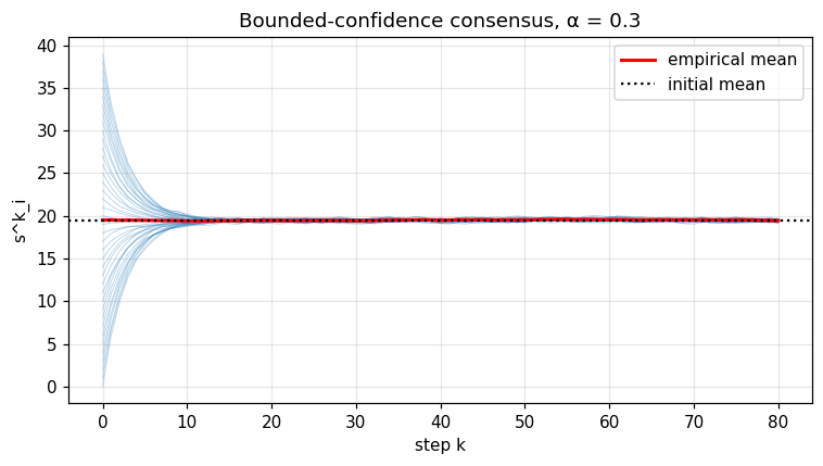
Mean conservation. Averaging the update over \(i\) gives \(\bar s^{k+1} = \bar s^k + \bar\xi^k\) with \(\mathbb{E}[\bar\xi^k] = 0\), so the empirical mean is a martingale and is exactly preserved in expectation:
In the noiseless case \(\sigma = 0\) the mean is preserved path-by-path.
Geometric contraction of the spread. Define the deviation \(d^k_i := s^k_i - \bar s^k\). The update implies
so in the absence of noise \(\| d^k \|_\infty \le (1 - \alpha)^k \| d^0 \|_\infty\) — the spread contracts geometrically with rate \(1 - \alpha\). The companion notebook plots \(\max_i s^k_i - \min_i s^k_i\) on a log scale across \(\alpha \in \{0.05, \dots, 1\}\) and recovers exactly this slope.
Stationary variance with noise. Treating the deviation as an AR(1) process with input variance \(\sigma^2 (1 - 1/N)\), the steady-state variance of any single agent’s deviation is
Continuous-time limit (linear Vlasov). Sending \(\alpha = \theta\, \Delta t\), \(\xi^k_i = \sigma \sqrt{\Delta t}\, W^i_k\) and \(\Delta t \to 0\) recovers the McKean–Vlasov SDE \(dX^i_t = \theta(\bar X_t - X^i_t)\, dt + \sigma\, dW^i_t\) of McKean–Vlasov — propagation of chaos — the discrete consensus update is the prototype of mean-field interaction.
Spectral interpretation. On a general weighted graph the update reads \(s^{k+1} = (I - \alpha L)\, s^k + \xi^k\), where \(L\) is the normalised Laplacian. The complete-graph case shipped here has \(L = I - \tfrac1N \mathbf{1}\mathbf{1}^\top\) with eigenvalue \(1\) on the orthogonal complement of \(\mathbf{1}\), hence the contraction rate \(1 - \alpha\) above. Replacing \(\mathbf{1}\mathbf{1}^\top / N\) by an arbitrary stochastic matrix produces the full DeGroot model and is a one-liner extension on the Rust side.
Why it matters
Opinion dynamics & social learning. Calibration of polarisation/consensus models (Bayesian persuasion, social media echo chambers, voting-system stability).
Distributed estimation & federated learning. Average-consensus protocols for sensor networks, gossip algorithms, federated averaging — all reduce to the same contraction argument with explicit convergence rate \(1 - \alpha\).
Coupled-oscillator physics. Linear approximation of the Kuramoto / Vicsek models near the synchronised regime; direct comparison with the McKean–Vlasov continuous limit.
Note
📓 Companion notebook — view on GitHub · download .ipynb
15 — Agent-based dynamics
import numpy as np
import matplotlib.pyplot as plt
from optimizr import _core as opt
plt.rcParams['figure.figsize'] = (7, 4)
plt.rcParams['figure.dpi'] = 110
init = np.arange(40.0).tolist()
init_mean = float(np.mean(init))
res = opt.consensus_dynamics(init, alpha=0.3, noise_sigma=0.1,
                              n_steps=80, seed=0)
n_t = res['n_steps']; n_a = res['n_agents']
S = np.array(res['states_flat']).reshape(n_t, n_a)
mean_traj = np.array(res['mean_trajectory'])
print('initial mean =', init_mean)
print('final mean   =', mean_traj[-1])
print('final std    =', float(S[-1].std()))
fig, ax = plt.subplots()
for i in range(n_a):
    ax.plot(S[:, i], color='tab:blue', alpha=0.3, lw=0.6)
ax.plot(mean_traj, color='red', lw=2, label='empirical mean')
ax.axhline(init_mean, color='k', ls=':', label='initial mean')
ax.set_xlabel('step k'); ax.set_ylabel('s^k_i'); ax.legend(); ax.grid(alpha=0.3)
ax.set_title('Bounded-confidence consensus, α = 0.3')
fig.tight_layout(); plt.show()

fig, ax = plt.subplots()
for alpha in [0.05, 0.1, 0.3, 0.6, 1.0]:
    r = opt.consensus_dynamics(init, alpha=alpha, noise_sigma=0.0, n_steps=60, seed=0)
    S = np.array(r['states_flat']).reshape(r['n_steps'], r['n_agents'])
    spread = S.max(axis=1) - S.min(axis=1)
    ax.semilogy(spread, label=f'α = {alpha:g}')
ax.set_xlabel('step k'); ax.set_ylabel('max_i s − min_i s')
ax.set_title('Convergence rate vs averaging weight α'); ax.legend(); ax.grid(alpha=0.3)
fig.tight_layout(); plt.show()

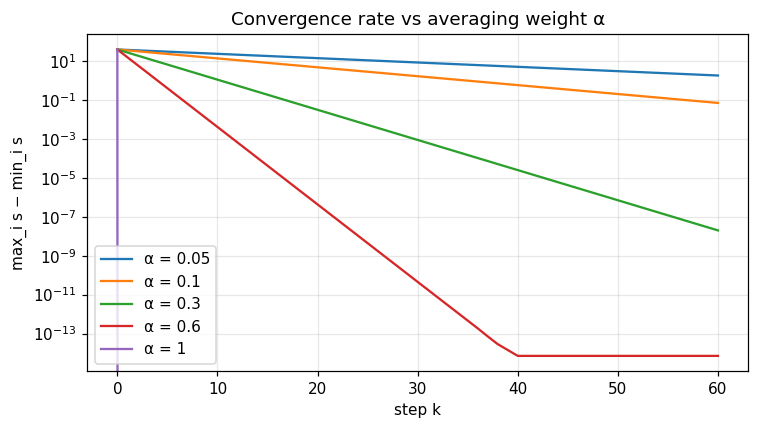
Verified: without noise, the empirical mean is exactly preserved and the spread decays geometrically.
API
pub fn simulate_agent_based<T>(initial: &[f64], transition: T, cfg: &AgentBasedConfig) -> Result<AgentBasedResult>
where T: Fn(f64, &[f64], usize) -> f64;

pub struct AgentBasedConfig { pub n_agents: usize, pub n_steps: usize, pub noise_sigma: f64, pub seed: u64 }
pub struct AgentBasedResult { pub states: Array2<f64>, pub mean_trajectory: Array1<f64> }