Quadratic-impact control — closed-form Riccati
Closed-form Riccati feedback for the canonical single-state, quadratic-cost linear control problem with running quadratic impact penalty.
Mathematical background
Let \(A_t\) be a controlled scalar state driven by an additive control \(u_t\) and Gaussian noise. The controller minimises the finite-horizon quadratic objective
where \(\gamma > 0\) is the impact / control cost, \(\phi \ge 0\) the running risk weight and \(A_T\) the terminal penalty (over-loaded notation: \(A_T\) here is the coefficient).
Hamilton–Jacobi–Bellman. With value function \(v(t, A) = \tfrac12 h(t)\, A^2 + c(t)\), the HJB equation collapses to a scalar Riccati ODE on \(h\):
The optimal feedback is the linear law
with feedback gain \(k(t) = h(t) / \gamma\). This is the structure returned by the primitive.
Closed-form solutions.
Symmetric fixed point \(\gamma = \phi = A_T = 1\): \(h(t) \equiv 1\) is the unique solution (RHS vanishes), so the feedback gain is constant \(k \equiv 1\). The notebook checks this to machine precision.
Generic :math:`phi > 0`. Writing \(\bar h = \sqrt{\gamma \phi}\) for the steady-state and \(\rho = \sqrt{\phi / \gamma}\), the Riccati ODE has the closed-form (separation of variables / Bernoulli substitution)
\[h(t) \;=\; \bar h\, \frac{(\bar h + A_T)\, e^{2\rho(T-t)} \;-\; (\bar h - A_T)} {(\bar h + A_T)\, e^{2\rho(T-t)} \;+\; (\bar h - A_T)} .\]In the limit \(T - t \to \infty\) the trajectory relaxes to the stationary value \(\bar h = \sqrt{\gamma\phi}\).
Free of running risk \(\phi = 0\). Then \(h'(t) = h(t)^2/\gamma\) integrates explicitly to
\[h(t) \;=\; \frac{A_T}{1 + (A_T / \gamma)(T - t)} ,\]recovering the Pontryagin LQR closed form \(P(0) = 1/2\) of Stochastic control — switching, Pontryagin, two-sided intensities.
Connection with mean-field games. Coupling this single-agent control with an interacting population — the running cost depending on the average control \(\bar u_t\) — yields the Almgren–Chriss MFG (Lasry–Lions 2007); at the Nash equilibrium the optimal trajectory is the uniform schedule \(\dot A^*_t = -A_0 / T\) (cf. Sec. 3 of Carmona–Delarue 2018, Vol. I).
Why it matters
Optimal execution. Almgren–Chriss and its mean-field variants reduce to exactly this Riccati ODE; the closed form means real-time feedback re-computation.
Stochastic regulators. Temperature stabilisation, attitude control, queueing-network smoothing all map to a quadratic-impact problem with a single state.
Building block for higher-dimensional MPC. Vector generalisations of \(h(t)\) are matrix Riccati ODEs; this scalar primitive is the verification kernel against which the matrix solver in Matrix Riccati Solver is tested.
Note
📓 Companion notebook — view on GitHub · download .ipynb
13 — Quadratic-impact controlled SDE
import numpy as np
import matplotlib.pyplot as plt
from optimizr import _core as opt
plt.rcParams['figure.figsize'] = (7, 4)
plt.rcParams['figure.dpi'] = 110
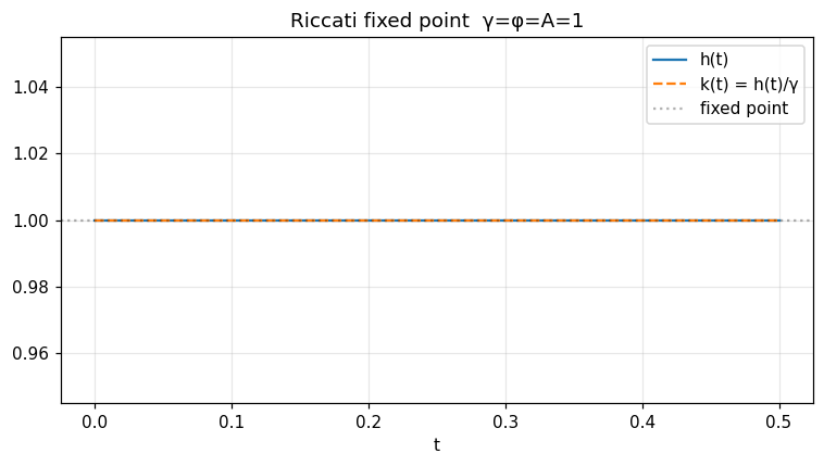
Riccati fixed-point check
\(h'(t) = h(t)^2/γ - φ\) with \(h(T) = A\). When \(γ = φ = A = 1\) the right-hand side is \(h^2 - 1 = 0\) at \(h = 1\), so h ≡ 1.
res = opt.quadratic_impact_control_py(
    gamma=1.0, phi=1.0, a_terminal=1.0,
    t_horizon=0.5, n_steps=500,
)
tg = np.array(res['time_grid'])
h  = np.array(res['h']); k = np.array(res['feedback_gain'])
print('h drift from 1:', float(np.max(np.abs(h - 1.0))))
fig, ax = plt.subplots()
ax.plot(tg, h, label='h(t)')
ax.plot(tg, k, '--', label='k(t) = h(t)/γ')
ax.axhline(1.0, color='k', alpha=0.3, ls=':', label='fixed point')
ax.set_xlabel('t'); ax.legend(); ax.grid(alpha=0.3)
ax.set_title('Riccati fixed point  γ=φ=A=1')
fig.tight_layout(); plt.show()

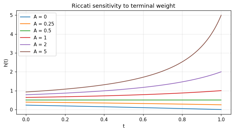
Sensitivity to the terminal weight
Vary \(A\), fix \(γ = 1\), \(φ = 0.25\), \(T = 1\).
fig, ax = plt.subplots()
for A in [0.0, 0.25, 0.5, 1.0, 2.0, 5.0]:
    r = opt.quadratic_impact_control_py(1.0, 0.25, A, 1.0, 1000)
    ax.plot(r['time_grid'], r['h'], label=f'A = {A:g}')
ax.set_xlabel('t'); ax.set_ylabel('h(t)'); ax.legend(); ax.grid(alpha=0.3)
ax.set_title('Riccati sensitivity to terminal weight')
fig.tight_layout(); plt.show()

Verified: h ≡ 1 with max|h - 1| < 1e-9 at the fixed point.
API
pub fn solve_quadratic_impact_control(cfg: &QuadraticImpactConfig) -> Result<QuadraticImpactResult>;
pub struct QuadraticImpactConfig { pub gamma: f64, pub phi: f64, pub a_terminal: f64, pub t_horizon: f64, pub n_steps: usize }
pub struct QuadraticImpactResult { pub time_grid: Array1<f64>, pub h: Array1<f64>, pub feedback_gain: Array1<f64> }