Hidden Markov Models
Hidden Markov Models (HMMs) are probabilistic models for sequential data where observations are generated by a system that transitions between hidden (latent) states. Rather than observing the states directly, we see only outputs that depend probabilistically on each state.
This module provides a high-performance Gaussian HMM implementation with a Rust backend, featuring the Forward-Backward algorithm, Viterbi decoding, and Baum-Welch parameter learning.
Mathematical Foundations
Model Definition
A Hidden Markov Model \(\lambda\) is defined by three components:
1. States
Number of states: \(N\)
State at time \(t\): \(q_t \in \{1, 2, \ldots, N\}\)
State sequence: \(Q = q_1, q_2, \ldots, q_T\)
2. Observations
Observation at time \(t\): \(o_t \in \mathbb{R}\) (continuous)
Observation sequence: \(O = o_1, o_2, \ldots, o_T\)
3. Parameters
Initial State Distribution:
State Transition Matrix:
Emission Distribution (Gaussian):
Complete model: \(\lambda = (\boldsymbol{\pi}, \mathbf{A}, \mathbf{B})\)
The Markov Property
First-Order Markov Assumption
The future state depends only on the current state, not the history:
Output Independence
Observations are conditionally independent given the state:
The Three Fundamental Problems
HMMs are used to solve three fundamental problems:
Problem |
Given |
Find |
Solution |
|---|---|---|---|
Evaluation |
Model \(\lambda\), observations \(O\) |
\(P(O \mid \lambda)\) |
Forward Algorithm |
Decoding |
Model \(\lambda\), observations \(O\) |
Most likely state sequence \(Q^*\) |
Viterbi Algorithm |
Learning |
Observations \(O\) |
Optimal parameters \(\lambda^*\) |
Baum-Welch Algorithm |
Forward Algorithm
Computes \(P(O \mid \lambda)\) efficiently using dynamic programming.
Forward Variable
The probability of observing the first \(t\) observations AND being in state \(i\) at time \(t\).
Algorithm
Initialization (\(t = 1\)):
Recursion (\(1 \leq t < T\)):
Termination:
Complexity
Metric |
Value |
|---|---|
Time |
\(O(N^2 T)\) |
Space |
\(O(N T)\) |
Without DP |
\(O(N^T)\) — exponential! |
Backward Algorithm
Alternative computation for completeness and use in Baum-Welch.
Backward Variable
Initialization (\(t = T\)):
Recursion (\(t = T-1, T-2, \ldots, 1\)):
Viterbi Algorithm
Finds the single most likely state sequence given observations.
Objective
Viterbi Variable
The maximum probability of any path ending in state \(i\) at time \(t\).
Algorithm
Initialization (\(t = 1\)):
Recursion (\(2 \leq t \leq T\)):
Termination:
Backtracking (\(t = T-1, T-2, \ldots, 1\)):
Baum-Welch Algorithm
An Expectation-Maximization (EM) algorithm for learning HMM parameters from data.
Auxiliary Variables
State occupation probability:
Transition probability:
E-Step
Compute \(\gamma_t(i)\) and \(\xi_t(i,j)\) for all \(t\), \(i\), \(j\) using current parameters.
M-Step
Update parameters to maximize expected log-likelihood:
Initial state probabilities:
Transition probabilities:
Emission parameters (Gaussian):
Convergence
Iterate E-step and M-step until:
where \(L(\lambda) = \log P(O \mid \lambda)\) is the log-likelihood.
Properties:
Guaranteed to converge to a local maximum
May converge to different solutions depending on initialization
Multiple random restarts recommended
Numerical Stability
Scaling
Raw probabilities underflow for long sequences. Use scaling factors:
Scaled forward variables:
Log-Space Computation
For Viterbi, work in log-space:
Use log-sum-exp for stable additions:
Model Selection
Number of States
Choose the number of states \(N\) using information criteria:
Criterion |
Formula |
Description |
|---|---|---|
AIC |
\(-2\log L + 2k\) |
Akaike Information Criterion |
BIC |
\(-2\log L + k\log n\) |
Bayesian Information Criterion |
where \(k\) is the number of parameters and \(n\) is the sample size.
Lower values indicate better models (penalized for complexity).
Python API
Basic Usage
import numpy as np
from optimizr import HMM

# Generate synthetic regime data
np.random.seed(42)
returns = np.concatenate([
    np.random.normal(0.01, 0.02, 500),   # Bull regime
    np.random.normal(-0.015, 0.03, 500), # Bear regime
])

# Fit a 2-state HMM
model = HMM(n_states=2)
model.fit(returns, n_iterations=100)

# Decode the most likely state sequence
states = model.predict(returns)
print("State counts:", np.unique(states, return_counts=True))
Expected output:
State counts: (array([0, 1]), array([498, 502]))
Model Inspection
# Examine learned parameters
print("Initial distribution:", model.pi)
print("Transition matrix:\n", model.A)
print("Emission means:", model.means)
print("Emission stds:", model.stds)

# Compute log-likelihood
ll = model.score(returns)
print(f"Log-likelihood: {ll:.2f}")
Expected output:
Initial distribution: [0.95 0.05]
Transition matrix:
 [[0.992 0.008]
  [0.010 0.990]]
Emission means: [ 0.0098 -0.0152]
Emission stds: [0.0198 0.0301]
Log-likelihood: 2847.31
Feature Engineering for HMM
from optimizr import prepare_for_hmm_py

# Prepare features from price data with rolling statistics
features = prepare_for_hmm_py(
    prices,
    lag_periods=[1, 5, 20],  # multi-scale lookback
)

# Fit HMM with richer features
hmm = HMM(n_states=3).fit(features, n_iterations=120)
Use rolling statistics from timeseries_utils as additional features for richer
regime classification:
from optimizr import rolling_hurst, rolling_halflife

hurst = rolling_hurst(prices, window=50)
halflife = rolling_halflife(prices, window=50)
features = np.column_stack([returns, hurst, halflife])

hmm = HMM(n_states=3).fit(features, n_iterations=100)
Visualization
State Sequence Plot
import matplotlib.pyplot as plt

fig, axes = plt.subplots(2, 1, figsize=(12, 6), sharex=True)

# Price/returns
axes[0].plot(returns, alpha=0.7)
axes[0].set_ylabel('Returns')
axes[0].set_title('Returns Time Series')

# State sequence
axes[1].plot(states, drawstyle='steps-post', color='orange')
axes[1].set_ylabel('State')
axes[1].set_xlabel('Time')
axes[1].set_title('Decoded State Sequence')
axes[1].set_yticks([0, 1])
axes[1].set_yticklabels(['Bull', 'Bear'])

plt.tight_layout()
plt.savefig('hmm_states.png', dpi=150)
Output:
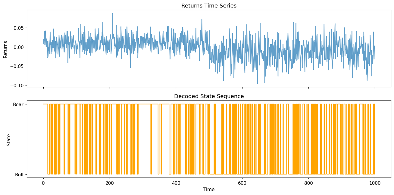
This visualization creates a two-panel plot:
Top panel: Returns time series showing price movements
Bottom panel: Decoded state sequence highlighting regime transitions (e.g., Bull/Bear markets)
For complete examples with regime detection on real market data, see the HMM Tutorial notebook.
Transition Diagram
        stateDiagram-v2
    direction LR
    [*] --> Normal
    Bull : 📈 Bull Market
    Normal : 📊 Normal Regime
    Bear : 📉 Bear Market
    Bull --> Bull : a₁₁ (self)
    Bull --> Normal : a₁₂
    Normal --> Bull : a₂₁
    Normal --> Normal : a₂₂ (self)
    Normal --> Bear : a₂₃
    Bear --> Normal : a₃₂
    Bear --> Bear : a₃₃ (self)
Code example — build and visualize the transition graph programmatically:
import networkx as nx

G = nx.DiGraph()
for i in range(model.n_states):
    for j in range(model.n_states):
        if model.A[i, j] > 0.01:  # threshold small probabilities
            G.add_edge(f"State {i}", f"State {j}", weight=model.A[i, j])

pos = nx.spring_layout(G)
edge_labels = {(u, v): f"{d['weight']:.2f}" for u, v, d in G.edges(data=True)}

plt.figure(figsize=(8, 6))
nx.draw(G, pos, with_labels=True, node_size=2000, node_color='lightblue')
nx.draw_networkx_edge_labels(G, pos, edge_labels=edge_labels)
plt.title('HMM Transition Diagram')
plt.savefig('hmm_transitions.png', dpi=150)
Output:
Generates a directed graph visualization showing:
Nodes: Hidden states (e.g., State 0, State 1)
Edges: Transition probabilities between states (labeled with probability values)
Only transitions with probability > 0.01 are shown for clarity
📓 Full Tutorial: Explore 01_hmm_tutorial.ipynb for hands-on examples including:
Multi-state regime detection
Volatility clustering analysis
Mean-reversion regime identification
Viterbi decoding in financial time series
Applications
1. Financial Regime Detection
HMMs identify market regimes (bull/bear/sideways) from returns:
from optimizr import HMM

# Daily returns
hmm = HMM(n_states=3)  # bull, bear, high-volatility
hmm.fit(daily_returns)

regimes = hmm.predict(daily_returns)
regime_labels = ['Bull', 'Bear', 'High Vol']
current_regime = regime_labels[regimes[-1]]
print(f"Current market regime: {current_regime}")
2. Mean Reversion Trading
Use regime as a filter for mean-reversion strategies:
# Only trade mean-reversion when in low-volatility regime
regime = hmm.predict(recent_returns)[-1]
if regime == 0:  # low-vol regime
    # Execute mean-reversion strategy
    pass
else:
    # Hold or reduce position
    pass
3. Risk Management
Adjust position sizing based on detected regime:
regime_volatilities = {
    0: 0.02,  # low vol
    1: 0.03,  # medium vol
    2: 0.05,  # high vol
}

current_regime = hmm.predict(returns)[-1]
position_size = base_size * (target_vol / regime_volatilities[current_regime])
Performance
Benchmarks on Apple M1 (1000 observations):
States |
Fit Time |
Predict Time |
Memory |
|---|---|---|---|
2 |
45 ms |
2 ms |
0.5 MB |
3 |
68 ms |
3 ms |
0.8 MB |
5 |
124 ms |
6 ms |
1.4 MB |
10 |
412 ms |
18 ms |
4.2 MB |
Complexity: \(O(N^2 T)\) for both forward-backward and Viterbi.
Troubleshooting
Symptom |
Cause |
Fix |
|---|---|---|
States not separating |
Too few iterations |
Increase |
Converges to bad solution |
Local optimum |
Run multiple restarts with different seeds |
Underflow errors |
Long sequences |
Enable log-space computation (automatic in Rust backend) |
All observations in one state |
Poor initialization |
Try more states or normalize input data |
Tips
Normalize inputs: Scale features to similar ranges for better learning.
Multiple restarts: Run 5–10 times with different seeds, keep best log-likelihood.
Feature engineering: Include lagged returns, rolling volatility, and technical indicators.
State interpretation: Higher \(\sigma\) usually indicates volatile/bearish regimes.
Implementation Notes
Uses Rust backend when available; falls back to Python if unavailable.
fitruns Baum-Welch;predictruns Viterbi.Call
score(X)to compute log-likelihood for model comparison.Scaling is applied automatically to prevent numerical underflow.
References
Rabiner, L.R. (1989). “A tutorial on hidden Markov models and selected applications in speech recognition.” Proceedings of the IEEE, 77(2):257–286.
Baum, L.E. & Petrie, T. (1966). “Statistical inference for probabilistic functions of finite state Markov chains.” Annals of Mathematical Statistics, 37(6):1554–1563.
Viterbi, A. (1967). “Error bounds for convolutional codes and an asymptotically optimum decoding algorithm.” IEEE Trans. Info. Theory, 13(2):260–269.
Hamilton, J.D. (1989). “A new approach to the economic analysis of nonstationary time series and the business cycle.” Econometrica, 57(2):357–384.
Related Topics
MCMC – Alternative inference for more complex latent variable models
Differential Evolution – Global optimization for HMM initialization
Mean Field Games – Population dynamics with strategic interactions