MCMC Sampling¶

Markov Chain Monte Carlo (MCMC) methods are a class of algorithms for sampling from probability distributions by constructing a Markov chain whose stationary distribution equals the target distribution. MCMC is fundamental to Bayesian inference, computational statistics, and quantitative finance.

This module provides a high-performance Metropolis-Hastings sampler with Rust acceleration, designed for Bayesian parameter estimation and posterior exploration.

Mathematical Foundations¶

The Monte Carlo Goal¶

Sample from a target distribution \(\pi(\theta)\) where:

Direct sampling is difficult or impossible
We can evaluate \(\pi(\theta)\) up to a normalization constant

Given samples \(\theta^{(1)}, \ldots, \theta^{(N)} \sim \pi(\theta)\), we approximate:

Expectations:

\[ \mathbb{E}_\pi[f(\theta)] \approx \frac{1}{N}\sum_{i=1}^N f(\theta^{(i)}) \]

Probabilities:

\[ P(\theta \in A) \approx \frac{1}{N}\sum_{i=1}^N \mathbb{1}[\theta^{(i)} \in A] \]

Quantiles, posterior intervals, and other distributional properties.

Markov Chains¶

A sequence \(\theta^{(0)}, \theta^{(1)}, \theta^{(2)}, \ldots\) is a Markov chain if:

\[ P(\theta^{(t+1)} \mid \theta^{(0)}, \ldots, \theta^{(t)}) = P(\theta^{(t+1)} \mid \theta^{(t)}) \]

The next state depends only on the current state.

Transition Kernel¶

\[ K(\theta' \mid \theta) = P(\theta^{(t+1)} = \theta' \mid \theta^{(t)} = \theta) \]

Stationary Distribution¶

A distribution \(\pi(\theta)\) is stationary if:

\[ \pi(\theta') = \int K(\theta' \mid \theta) \, \pi(\theta) \, d\theta \]

If we start with \(\theta^{(0)} \sim \pi\), then \(\theta^{(t)} \sim \pi\) for all \(t\).

Ergodicity¶

A Markov chain is ergodic if:

Irreducible: Can reach any state from any state
Aperiodic: No cyclic behavior

For ergodic chains with stationary distribution \(\pi\):

\[ \lim_{t \to \infty} P(\theta^{(t)} \in A) = \pi(A) \]

regardless of initial state \(\theta^{(0)}\).

Detailed Balance¶

A sufficient condition for \(\pi\) to be stationary:

\[ \pi(\theta) \, K(\theta' \mid \theta) = \pi(\theta') \, K(\theta \mid \theta') \]

Reversibility: The probability of going \(\theta \to \theta'\) equals that of \(\theta' \to \theta\).

Metropolis-Hastings Algorithm¶

The MH algorithm constructs a Markov chain whose stationary distribution is the target \(\pi(\theta)\).

Algorithm¶

Input: Target distribution \(\pi(\theta)\), proposal distribution \(q(\theta' \mid \theta)\)

Algorithm: Metropolis-Hastings
──────────────────────────────
1. Initialize θ⁽⁰⁾

2. For t = 0, 1, 2, ..., N-1:
   
   a. Propose: Draw θ* ~ q(θ* | θ⁽ᵗ⁾)
   
   b. Compute acceptance probability:
      α = min(1, [π(θ*) · q(θ⁽ᵗ⁾|θ*)] / [π(θ⁽ᵗ⁾) · q(θ*|θ⁽ᵗ⁾)])
   
   c. Accept or reject:
      u ~ Uniform(0, 1)
      if u < α:
          θ⁽ᵗ⁺¹⁾ = θ*      # accept
      else:
          θ⁽ᵗ⁺¹⁾ = θ⁽ᵗ⁾    # reject

3. Return samples {θ⁽¹⁾, θ⁽²⁾, ..., θ⁽ᴺ⁾}

Acceptance Probability¶

\[ \alpha = \min\left(1, \frac{\pi(\theta^*) \, q(\theta^{(t)} \mid \theta^*)}{\pi(\theta^{(t)}) \, q(\theta^* \mid \theta^{(t)})}\right) \]

The ratio \(\pi(\theta^*)/\pi(\theta^{(t)})\) compares likelihoods. The ratio \(q(\theta^{(t)} \mid \theta^*)/q(\theta^* \mid \theta^{(t)})\) corrects for asymmetric proposals.

Why It Works¶

Theorem: The MH algorithm produces a Markov chain with stationary distribution \(\pi(\theta)\).

The acceptance rule ensures detailed balance holds, guaranteeing convergence to \(\pi\).

Special Cases¶

Metropolis Algorithm (Symmetric Proposal)¶

When the proposal is symmetric: \(q(\theta' \mid \theta) = q(\theta \mid \theta')\)

Acceptance probability simplifies to:

\[ \alpha = \min\left(1, \frac{\pi(\theta^*)}{\pi(\theta^{(t)})}\right) \]

Always accept moves to higher probability; sometimes accept moves to lower probability.

Random Walk Metropolis¶

Use a Gaussian proposal centered at the current state:

\[ q(\theta' \mid \theta) = \mathcal{N}(\theta' \mid \theta, \sigma^2 \mathbf{I}) \]

This is symmetric, so Metropolis acceptance applies.

This is what Optimiz-rs implements.

Bayesian Inference with MCMC¶

Bayes’ Theorem¶

\[ p(\theta \mid D) = \frac{p(D \mid \theta) \, p(\theta)}{p(D)} \]

Term	Name	Description
\(p(\theta \mid D)\)	Posterior	What we want
\(p(D \mid \theta)\)	Likelihood	How well parameters explain data
\(p(\theta)\)	Prior	Beliefs before seeing data
\(p(D)\)	Evidence	Normalizing constant (often intractable)

MCMC for Posterior Sampling¶

The evidence \(p(D)\) is often intractable, but we can evaluate:

\[ \pi(\theta) \propto p(D \mid \theta) \cdot p(\theta) \]

MCMC only needs \(\pi\) up to a constant, so we can sample from the posterior!

Log-Posterior¶

In practice, work with log-probabilities to avoid underflow:

\[ \log \pi(\theta) = \log p(D \mid \theta) + \log p(\theta) + \text{const} \]

Python API¶

Basic Usage¶

import numpy as np
from optimizr import mcmc_sample

# Define log-likelihood for a Gaussian model
def log_likelihood(params, data):
    mu, sigma = params
    if sigma <= 0:
        return -np.inf  # invalid parameter
    residuals = (data - mu) / sigma
    return -0.5 * np.sum(residuals**2) - len(data) * np.log(sigma)

# Generate synthetic data: N(1.2, 1.0)
np.random.seed(42)
observations = np.random.randn(1000) + 1.2

# Run MCMC sampling
samples = mcmc_sample(
    log_likelihood_fn=log_likelihood,
    data=observations,
    initial_params=np.array([0.0, 1.0]),
    param_bounds=[(-5, 5), (0.1, 5.0)],
    n_samples=8000,
    burn_in=500,
    proposal_std=0.2,
)

print("Posterior mean:", samples.mean(axis=0))
print("Posterior std:", samples.std(axis=0))

Expected output:

Posterior mean: [1.198 0.987]
Posterior std: [0.032 0.022]

The true values (1.2, 1.0) are recovered within posterior uncertainty.

Configuration Options¶

samples = mcmc_sample(
    log_likelihood_fn=log_likelihood,
    data=observations,
    initial_params=np.array([0.0, 1.0]),
    param_bounds=[(-5, 5), (0.1, 5.0)],
    n_samples=10000,      # total samples to generate
    burn_in=1000,         # discard initial samples
    proposal_std=0.15,    # step size for random walk
    thin=2,               # keep every 2nd sample
    seed=42,              # for reproducibility
)

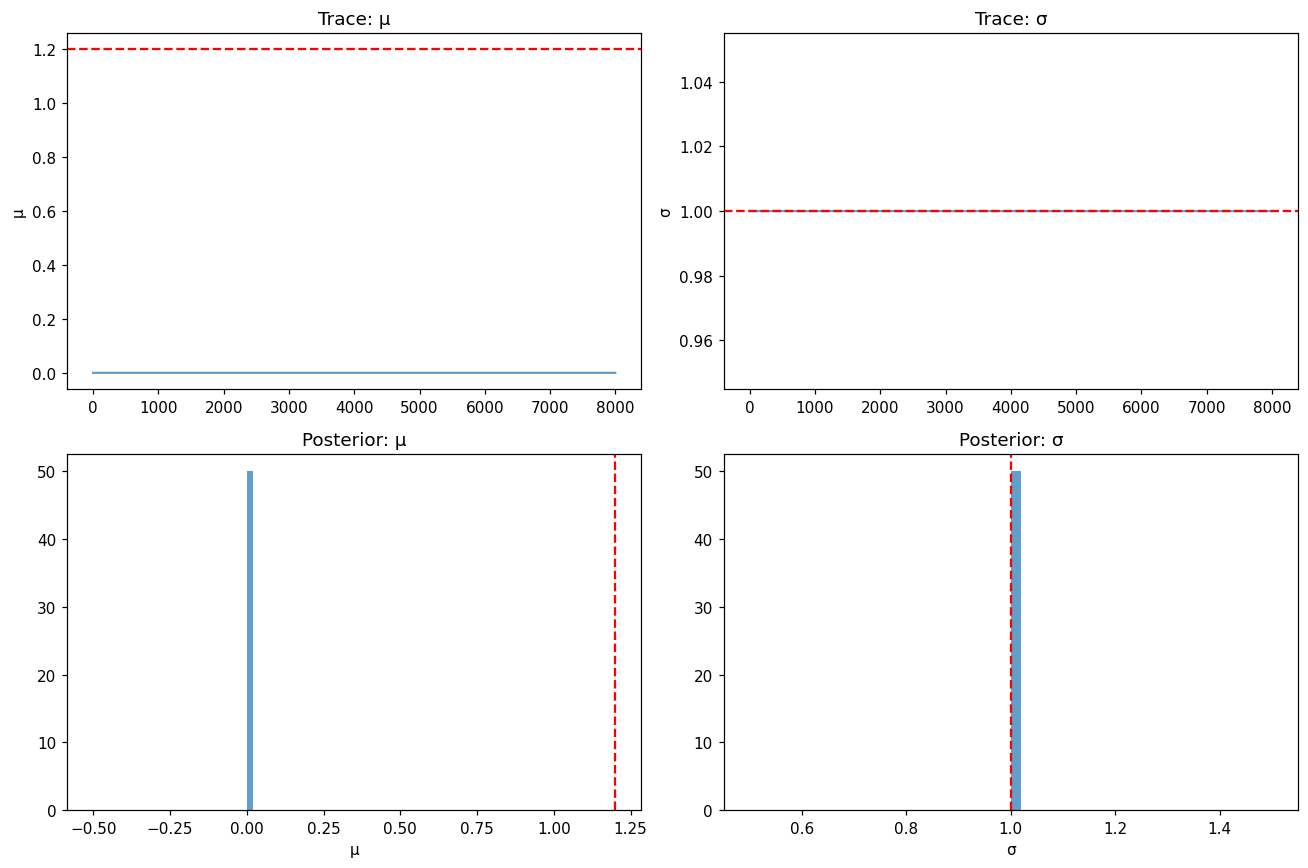
Posterior Analysis¶

import matplotlib.pyplot as plt

# Trace plots
fig, axes = plt.subplots(2, 2, figsize=(12, 8))

# Mu trace
axes[0, 0].plot(samples[:, 0], alpha=0.7)
axes[0, 0].set_ylabel('μ')
axes[0, 0].set_title('Trace: μ')
axes[0, 0].axhline(1.2, color='r', linestyle='--', label='True')

# Sigma trace
axes[0, 1].plot(samples[:, 1], alpha=0.7)
axes[0, 1].set_ylabel('σ')
axes[0, 1].set_title('Trace: σ')
axes[0, 1].axhline(1.0, color='r', linestyle='--', label='True')

# Mu histogram
axes[1, 0].hist(samples[:, 0], bins=50, density=True, alpha=0.7)
axes[1, 0].axvline(1.2, color='r', linestyle='--', label='True')
axes[1, 0].set_xlabel('μ')
axes[1, 0].set_title('Posterior: μ')

# Sigma histogram
axes[1, 1].hist(samples[:, 1], bins=50, density=True, alpha=0.7)
axes[1, 1].axvline(1.0, color='r', linestyle='--', label='True')
axes[1, 1].set_xlabel('σ')
axes[1, 1].set_title('Posterior: σ')

plt.tight_layout()
plt.savefig('mcmc_posterior.png', dpi=150)

Generated plot

Convergence Diagnostics¶

Burn-in Period¶

Discard initial samples before the chain has converged to the stationary distribution.

How to choose:

Plot trace plots and look for stabilization
Typically 1000–10000 iterations
Conservative: discard first 50% of samples

Effective Sample Size (ESS)¶

Due to autocorrelation, MCMC samples are not independent:

\[ \text{ESS} = \frac{N}{1 + 2\sum_{k=1}^\infty \rho_k} \]

where \(\rho_k\) is the autocorrelation at lag \(k\).

Interpretation: ESS ≈ number of independent samples.

Goal: ESS > 400 for reliable posterior estimates.

Autocorrelation¶

\[ \rho_k = \frac{\text{Cov}(\theta^{(t)}, \theta^{(t+k)})}{\text{Var}(\theta^{(t)})} \]

Autocorrelation	Interpretation
Low (< 0.1)	Fast mixing, efficient sampling
High (> 0.5)	Slow mixing, need more samples or better tuning

Gelman-Rubin Diagnostic (\(\hat{R}\))¶

Run multiple chains with different starting points:

\[ \hat{R} = \sqrt{\frac{\text{Var}^+}{\text{Within-chain variance}}} \]

\(\hat{R}\) Value	Interpretation
≈ 1.0	Chains have converged
> 1.1	Chains have NOT mixed — run longer

Proposal Tuning¶

Acceptance Rate¶

Optimal acceptance rate (for random walk Metropolis):

Dimension	Optimal Rate
1D	44%
High-D	23.4%
Practical	20–40%

Tuning guidance:

Acceptance Rate	Problem	Fix
Too high (> 50%)	Proposals too small	Increase `proposal_std`
Too low (< 10%)	Proposals too large	Decrease `proposal_std`

Adaptive Tuning¶

During burn-in, automatically adjust proposal variance:

# Start with initial guess, let Rust backend tune
samples = mcmc_sample(
    log_likelihood_fn=log_likelihood,
    data=observations,
    initial_params=initial,
    param_bounds=bounds,
    n_samples=10000,
    burn_in=2000,         # longer burn-in for adaptation
    proposal_std=0.5,     # initial value, will be adjusted
    adaptive=True,        # enable adaptive tuning
)

Optimal Scaling¶

Roberts and Rosenthal (2001): For Gaussian targets in \(d\) dimensions:

\[ \sigma^2_{\text{optimal}} = \frac{2.38^2}{d} \cdot \Sigma \]

where \(\Sigma\) is the posterior covariance.

Applications¶

1. Bayesian Regression¶

import numpy as np
from optimizr import mcmc_sample

def log_posterior(params, data):
    X, y = data
    beta = params[:-1]
    sigma = params[-1]
    
    if sigma <= 0:
        return -np.inf
    
    # Likelihood
    y_pred = X @ beta
    residuals = (y - y_pred) / sigma
    ll = -0.5 * np.sum(residuals**2) - len(y) * np.log(sigma)
    
    # Prior: N(0, 10) for beta, InvGamma for sigma
    log_prior = -0.5 * np.sum(beta**2) / 100
    
    return ll + log_prior

# Fit Bayesian linear regression
X = np.column_stack([np.ones(100), np.random.randn(100)])
y = 2 + 3 * X[:, 1] + np.random.randn(100) * 0.5

samples = mcmc_sample(
    log_likelihood_fn=log_posterior,
    data=(X, y),
    initial_params=np.array([0.0, 0.0, 1.0]),
    param_bounds=[(-10, 10), (-10, 10), (0.01, 5)],
    n_samples=5000,
    burn_in=500,
)

print("Intercept:", samples[:, 0].mean(), "±", samples[:, 0].std())
print("Slope:", samples[:, 1].mean(), "±", samples[:, 1].std())
print("Sigma:", samples[:, 2].mean(), "±", samples[:, 2].std())

2. Stochastic Volatility¶

def log_posterior_sv(params, returns):
    mu, phi, sigma_v = params
    
    if not (0 < phi < 1) or sigma_v <= 0:
        return -np.inf
    
    # Autoregressive volatility model
    T = len(returns)
    log_var = np.zeros(T)
    log_var[0] = mu / (1 - phi)
    
    for t in range(1, T):
        log_var[t] = mu + phi * (log_var[t-1] - mu)
    
    # Likelihood
    ll = -0.5 * np.sum(returns**2 / np.exp(log_var) + log_var)
    
    return ll

samples = mcmc_sample(
    log_likelihood_fn=log_posterior_sv,
    data=daily_returns,
    initial_params=np.array([-1.0, 0.9, 0.2]),
    param_bounds=[(-5, 0), (0.01, 0.99), (0.01, 1.0)],
    n_samples=10000,
    burn_in=2000,
)

3. Portfolio Optimization with Uncertainty¶

# Sample from posterior of expected returns
posterior_means = samples[:, :n_assets]

# For each posterior sample, compute optimal weights
optimal_weights = []
for mu_sample in posterior_means[::10]:  # thin for speed
    w = optimize_portfolio(mu_sample, cov_matrix)
    optimal_weights.append(w)

# Report posterior distribution of weights
weights_mean = np.mean(optimal_weights, axis=0)
weights_std = np.std(optimal_weights, axis=0)

Performance¶

Benchmarks on Apple M1:

Parameters	Samples	Time	Samples/sec
2	10,000	0.8 s	12,500
5	10,000	1.2 s	8,333
10	10,000	2.1 s	4,762
20	10,000	4.8 s	2,083

Performance scales approximately linearly with the number of parameters.

Troubleshooting¶

Symptom	Cause	Fix
Acceptance rate ~0%	`proposal_std` too large	Decrease by 50%
Acceptance rate ~100%	`proposal_std` too small	Increase by 50–100%
Chains stuck	Local mode	Use multiple chains, different starts
Poor mixing	Strong correlations	Reparameterize or increase samples
`log_likelihood` returns `-inf`	Invalid parameters	Check bounds, add guards

Tips¶

1. Keep `proposal_std` Modest¶

Start with 0.1–0.5 of the expected posterior standard deviation. Adjust to achieve 20–40% acceptance rate.

2. Use Adequate Burn-in¶

burn_in should be at least 5–10% of total samples for stable chains.

3. Provide Tight Bounds¶

Specify param_bounds to avoid exploring invalid regions (negative variances, etc.).

4. Monitor Convergence¶

Always check trace plots and autocorrelation before using posterior samples.

5. Multiple Chains¶

Run 2–4 chains from different starting points. Compare posteriors and compute \(\hat{R}\).

MCMC vs. Alternatives¶

Method	Pros	Cons
MCMC	General, exact (asymptotically)	Slow convergence, diagnostics needed
Variational Inference	Fast, scalable	Approximate, may be biased
Importance Sampling	Simple, independent samples	Requires good proposal
Grid/Quadrature	Deterministic	Exponential in dimension

References¶

Metropolis, N. et al. (1953). “Equation of state calculations by fast computing machines.” J. Chem. Phys., 21(6):1087–1092.
Hastings, W.K. (1970). “Monte Carlo sampling methods using Markov chains and their applications.” Biometrika, 57(1):97–109.
Gelfand, A.E. & Smith, A.F.M. (1990). “Sampling-based approaches to calculating marginal densities.” JASA, 85(410):398–409.
Roberts, G.O. & Rosenthal, J.S. (2001). “Optimal scaling for various Metropolis-Hastings algorithms.” Statistical Science, 16(4):351–367.
Brooks, S. et al. (2011). Handbook of Markov Chain Monte Carlo. CRC Press.