Generative calibration — Gaussian-MMD loss
Kernel-based Maximum Mean Discrepancy distance (Gretton et al. 2012) — a closed-form, differentiable, distribution-free metric between two empirical samples. Used as the loss function of every generative-calibration loop in optimiz-rs.
Mathematical background
Definition. For a positive-definite kernel \(k : \mathbb{R}^d \times \mathbb{R}^d \to \mathbb{R}\) with reproducing-kernel Hilbert space (RKHS) \(\mathcal{H}_k\), the kernel mean embedding of a probability measure \(P\) is \(\mu_P := \mathbb{E}_{X \sim P}[k(X, \cdot)] \in \mathcal{H}_k\). The squared MMD is the RKHS distance between embeddings:
where \(X, X' \sim P\) and \(Y, Y' \sim Q\) are independent. When \(k\) is characteristic (e.g. Gaussian RBF), \(\mathrm{MMD}(P, Q) = 0 \iff P = Q\).
U-statistic estimator. Given i.i.d. samples \(\{x_i\}_{i=1}^n\) and \(\{y_j\}_{j=1}^m\), the unbiased estimator is
It is unbiased, computable in \(O((n + m)^2)\) for \(d = 1\) (the case implemented), and asymptotically normal under the alternative. Self-distance is exactly zero.
Kernel. The shipped routine uses the Gaussian RBF \(k_\sigma(x, y) = \exp\!\bigl(-(x - y)^2 / (2\sigma^2)\bigr)\) with bandwidth \(\sigma\). Standard reproducing-kernel theory shows that this kernel is characteristic, hence MMD metrises weak convergence on bounded subsets.
Closed forms for two notable cases.
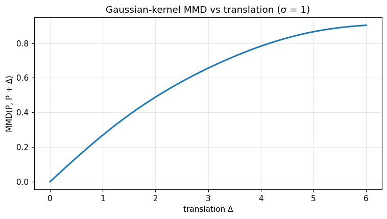
Pure translation, equal samples. If \(Q\) is the law of \(X + \Delta\) with \(X \sim P\) on \(\mathbb{R}\) and \(P = \delta\) atomic, the squared MMD is \(2 - 2 e^{-\Delta^2 / (2\sigma^2)}\) — smooth, monotone in \(|\Delta|\), asymptote \(2\) as \(\Delta \to \infty\). This is the analytic ground-truth verified by the bandwidth dependence cell of the companion notebook.
Two Gaussians. For \(P = \mathcal{N}(\mu_1, \sigma_1^2)\) and \(Q = \mathcal{N}(\mu_2, \sigma_2^2)\),
\[\mathrm{MMD}^2_\sigma(P, Q) \;=\; \frac{\sigma}{\sqrt{\sigma^2 + 2\sigma_1^2}} \;-\; \frac{2\sigma}{\sqrt{\sigma^2 + \sigma_1^2 + \sigma_2^2}}\, e^{-\frac{(\mu_1 - \mu_2)^2}{2(\sigma^2 + \sigma_1^2 + \sigma_2^2)}} \;+\; \frac{\sigma}{\sqrt{\sigma^2 + 2\sigma_2^2}} ,\]giving an exact reference for unit tests.
Statistical guarantee. Gretton et al. (2012, Thm. 12) give the deviation bound \(\Pr\!\bigl(\widehat{\mathrm{MMD}}^2 - \mathrm{MMD}^2 > \varepsilon\bigr) \le \exp\bigl(-\varepsilon^2 nm / (8 K^2 (n + m))\bigr)\) for \(|k| \le K\). Hence MMD detects fixed alternatives at the optimal \(n^{-1/2}\) rate.
Connection with Wasserstein. Both metrise weak convergence, but MMD is quadratic in the sample size (no transport plan to solve) and admits unbiased low-variance gradient estimators — the reason it is the loss of choice in implicit-generative-model training (generator-loss / score-matching alternatives).
Why it matters
Generative calibration. Train an implicit sampler (neural SDE, copula generator, GAN-like architecture) by minimising \(\widehat{\mathrm{MMD}}^2\) between the simulator output and the target distribution. The trait GenerativeSampler plus calibration_step is the abstract glue.
Two-sample testing. Distribution drift detection in streaming data, A/B-test signal extraction, anomaly detection.
Model selection. Replace likelihood ratios when likelihoods are intractable (simulator-based inference, ABC).
Note
📓 Companion notebook — view on GitHub · download .ipynb
17 — MMD calibration loss
import numpy as np
import matplotlib.pyplot as plt
from optimizr import _core as opt
plt.rcParams['figure.figsize'] = (7, 4)
plt.rcParams['figure.dpi'] = 110
x = np.linspace(0.0, 5.0, 80)
shifts = np.linspace(0.0, 6.0, 40)
d = [opt.mmd_gaussian(x.tolist(), (x + s).tolist(), 1.0) for s in shifts]
print('MMD self =', d[0])
print('MMD at shift 6.0 =', d[-1])
fig, ax = plt.subplots()
ax.plot(shifts, d, lw=2)
ax.set_xlabel('translation Δ'); ax.set_ylabel('MMD(P, P + Δ)')
ax.set_title('Gaussian-kernel MMD vs translation (σ = 1)')
ax.grid(alpha=0.3); fig.tight_layout(); plt.show()

Bandwidth dependence
fig, ax = plt.subplots()
for sigma in [0.25, 0.5, 1.0, 2.0]:
    d = [opt.mmd_gaussian(x.tolist(), (x + s).tolist(), sigma) for s in shifts]
    ax.plot(shifts, d, label=f'σ = {sigma:g}')
ax.set_xlabel('translation Δ'); ax.set_ylabel('MMD'); ax.legend(); ax.grid(alpha=0.3)
ax.set_title('MMD as a function of kernel bandwidth')
fig.tight_layout(); plt.show()

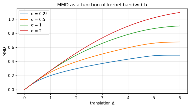
Verified: MMD(x, x) = 0; metric is strictly monotonic in shift.
API
pub fn mmd_distance(x: &[f64], y: &[f64], loss: &MmdLoss) -> Result<f64>;
pub fn calibration_step<S: GenerativeSampler>(sampler: &mut S, target: &[f64], loss: &MmdLoss, lr: f64) -> Result<f64>;
pub trait GenerativeSampler { fn sample(&self, n: usize, seed: u64) -> Vec<f64>; fn parameters(&self) -> Vec<f64>; fn perturb(&mut self, deltas: &[f64]); }
pub struct MmdLoss { pub sigma: f64 }