Grid Search¶

Grid Search (also called parameter sweep) is a deterministic hyperparameter optimization method that exhaustively evaluates all combinations of parameter values from a predefined grid. While simple, it provides guaranteed coverage of the search space and is ideal for low-dimensional problems.

This module provides a fast implementation with optional Rust acceleration for Cartesian product generation and parallel evaluation.

Mathematical Foundations¶

Problem Formulation¶

Given an objective function \(f(\theta)\) and a discrete parameter grid:

\[ \Theta = \Theta_1 \times \Theta_2 \times \cdots \times \Theta_D \]

where \(\Theta_i = \{\theta_{i,1}, \theta_{i,2}, \ldots, \theta_{i,n_i}\}\) is the set of candidate values for parameter \(i\).

Objective: Find the optimal parameters:

\[ \theta^* = \arg\min_{\theta \in \Theta} f(\theta) \]

Total Evaluations¶

The number of function evaluations grows as the Cartesian product:

\[ |\Theta| = \prod_{i=1}^{D} n_i \]

where \(n_i = |\Theta_i|\) is the number of values for parameter \(i\).

Parameters	Values Each	Total Evaluations
2	5	25
3	5	125
4	5	625
5	5	3,125
3	10	1,000
5	10	100,000

Warning: Grid search suffers from the curse of dimensionality. Use sparingly for \(D > 4\) or when function evaluations are expensive.

Algorithm¶

Algorithm: Grid Search
──────────────────────
Input: objective f, parameter grid Θ = Θ₁ × Θ₂ × ... × Θ_D

1. Generate all combinations: C = Θ₁ × Θ₂ × ... × Θ_D

2. Initialize: best_score = ∞, best_params = None

3. For each θ in C:
   a. Evaluate: score = f(θ)
   b. If score < best_score:
      best_score = score
      best_params = θ

4. Return best_params, best_score

When to Use Grid Search¶

Good Use Cases¶

✅ Few parameters (D ≤ 3–4)

✅ Coarse exploration before fine-tuning

✅ Discrete parameters (e.g., layer counts, categoricals)

✅ Reproducibility required (deterministic)

✅ Parameter interactions need full coverage

✅ Fast objectives (< 1 second per evaluation)

Poor Use Cases¶

❌ Many parameters (D > 5) — exponential explosion

❌ Continuous parameters — wastes evaluations between grid points

❌ Expensive objectives — better to use adaptive methods

❌ High-resolution search — consider random search or DE

Python API¶

Basic Usage¶

from optimizr import grid_search

# Objective returns a scalar score (lower is better)
def objective(params):
    lr = params["lr"]
    dropout = params["dropout"]
    # Simulate validation loss
    return (lr - 0.02)**2 + (dropout - 0.1)**2

best_params, best_score = grid_search(
    objective_fn=objective,
    param_grid={
        "lr": [0.005, 0.01, 0.02, 0.05, 0.1],
        "dropout": [0.0, 0.05, 0.1, 0.2, 0.3],
    },
)

print(f"Best parameters: {best_params}")
print(f"Best score: {best_score:.6f}")

Expected output:

Best parameters: {'lr': 0.02, 'dropout': 0.1}
Best score: 0.000000

With Verbose Logging¶

best_params, best_score = grid_search(
    objective_fn=objective,
    param_grid=param_grid,
    verbose=True,  # print progress
)

Output:

[1/25] lr=0.005, dropout=0.0 → score=0.0127
[2/25] lr=0.005, dropout=0.05 → score=0.0102
...
[15/25] lr=0.02, dropout=0.1 → score=0.0000 [BEST]
...

Parallel Evaluation¶

For independent, thread-safe objectives:

best_params, best_score = grid_search(
    objective_fn=objective,
    param_grid=param_grid,
    n_jobs=4,  # parallel workers
)

Note: Objective function must be thread-safe (no shared mutable state).

Grid Construction Strategies¶

Linear Grid¶

Evenly spaced values:

param_grid = {
    "lr": [0.001, 0.005, 0.01, 0.05, 0.1],  # linear
}

Logarithmic Grid¶

For parameters spanning orders of magnitude:

import numpy as np

param_grid = {
    "lr": list(np.logspace(-4, -1, 10)),  # 1e-4 to 1e-1
    "weight_decay": list(np.logspace(-5, -2, 8)),
}

Mixed Types¶

param_grid = {
    "lr": [0.001, 0.01, 0.1],           # continuous
    "batch_size": [16, 32, 64, 128],    # integer
    "optimizer": ["adam", "sgd", "rmsprop"],  # categorical
    "use_bn": [True, False],            # boolean
}

Practical Example: Neural Network Tuning¶

import numpy as np
from optimizr import grid_search

def train_and_evaluate(params):
    """
    Train a neural network with given hyperparameters
    and return validation loss.
    """
    lr = params["lr"]
    dropout = params["dropout"]
    hidden_size = params["hidden_size"]
    
    # Simulated training (replace with real training loop)
    # In practice: build model, train, return val_loss
    
    # Synthetic loss surface for demonstration
    loss = (
        (lr - 0.01)**2 / 0.001 +
        (dropout - 0.15)**2 / 0.01 +
        (hidden_size - 128)**2 / 10000
    )
    return loss + np.random.normal(0, 0.001)  # add noise

param_grid = {
    "lr": [0.001, 0.005, 0.01, 0.02, 0.05],
    "dropout": [0.0, 0.1, 0.2, 0.3],
    "hidden_size": [64, 128, 256],
}

print(f"Total combinations: {5 * 4 * 3} = 60")

best_params, best_score = grid_search(
    objective_fn=train_and_evaluate,
    param_grid=param_grid,
    verbose=True,
)

print(f"\nBest configuration:")
print(f"  Learning rate: {best_params['lr']}")
print(f"  Dropout: {best_params['dropout']}")
print(f"  Hidden size: {best_params['hidden_size']}")
print(f"  Validation loss: {best_score:.4f}")

Expected output:

Total combinations: 60
[1/60] lr=0.001, dropout=0.0, hidden_size=64 → score=0.1892
...
[32/60] lr=0.01, dropout=0.2, hidden_size=128 → score=0.0027 [BEST]
...

Best configuration:
  Learning rate: 0.01
  Dropout: 0.2
  Hidden size: 128
  Validation loss: 0.0027

Visualization¶

Results Heatmap¶

import matplotlib.pyplot as plt
import numpy as np

# Collect all results
results = {}
for lr in param_grid["lr"]:
    for dropout in param_grid["dropout"]:
        params = {"lr": lr, "dropout": dropout, "hidden_size": 128}
        results[(lr, dropout)] = train_and_evaluate(params)

# Create heatmap
lrs = param_grid["lr"]
dropouts = param_grid["dropout"]
Z = np.array([[results[(lr, d)] for d in dropouts] for lr in lrs])

plt.figure(figsize=(8, 6))
plt.imshow(Z, origin='lower', aspect='auto', cmap='viridis_r')
plt.colorbar(label='Loss')
plt.xticks(range(len(dropouts)), dropouts)
plt.yticks(range(len(lrs)), lrs)
plt.xlabel('Dropout')
plt.ylabel('Learning Rate')
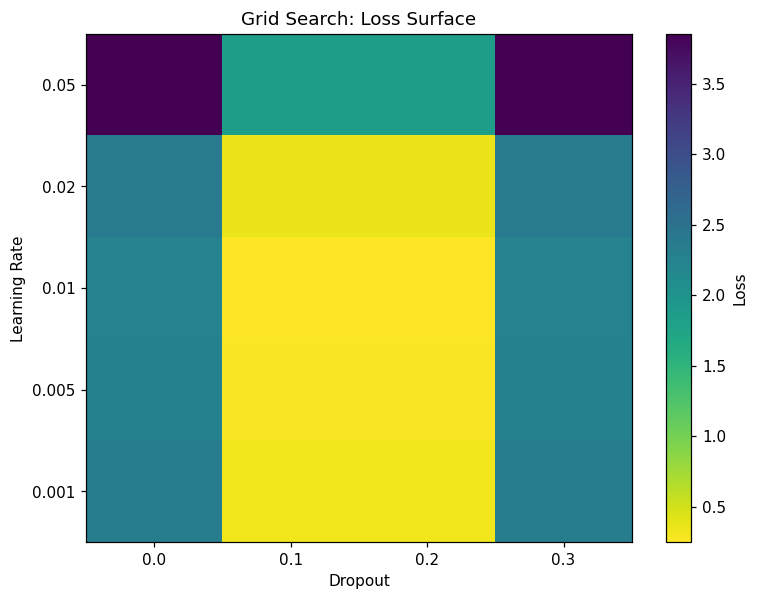
plt.title('Grid Search: Loss Surface')
plt.savefig('grid_search_heatmap.png', dpi=150)

Output:

Produces a 2D heatmap showing the loss landscape across different hyperparameter combinations:

X-axis: Dropout rate values
Y-axis: Learning rate values
Color intensity: Loss values (darker = lower loss = better performance)

This visualization helps identify optimal parameter regions and understand parameter interactions.

📓 Real-World Examples: See 04_real_world_applications.ipynb for grid search applied to:

Neural network hyperparameter tuning
Portfolio optimization
Trading strategy parameter selection

Combining with Other Methods¶

Coarse-to-Fine Search¶

Use grid search to identify promising regions, then refine:

from optimizr import grid_search, differential_evolution

# Step 1: Coarse grid search
coarse_grid = {
    "lr": [0.001, 0.01, 0.1],
    "dropout": [0.0, 0.2, 0.4],
}

coarse_best, _ = grid_search(objective, coarse_grid)
print(f"Coarse best: {coarse_best}")

# Step 2: Fine grid around best
fine_grid = {
    "lr": np.linspace(
        coarse_best["lr"] * 0.5,
        coarse_best["lr"] * 2,
        10
    ).tolist(),
    "dropout": np.linspace(
        max(0, coarse_best["dropout"] - 0.1),
        min(0.5, coarse_best["dropout"] + 0.1),
        10
    ).tolist(),
}

final_best, final_score = grid_search(objective, fine_grid)
print(f"Final best: {final_best}, score: {final_score:.6f}")

Warm-Start Differential Evolution¶

Use grid search results to seed DE:

from optimizr import grid_search, differential_evolution

# Quick grid search for initial region
best_grid, _ = grid_search(objective, coarse_grid)

# Initialize DE population around grid search result
bounds = [
    (best_grid["lr"] * 0.1, best_grid["lr"] * 10),
    (max(0, best_grid["dropout"] - 0.2), min(0.5, best_grid["dropout"] + 0.2)),
]

final_x, final_fx = differential_evolution(
    objective_fn=lambda x: objective({"lr": x[0], "dropout": x[1]}),
    bounds=bounds,
    maxiter=100,
)

Performance Comparison¶

Method	Evaluations	Coverage	Best For
Grid Search	\(\prod n_i\) (exponential)	Complete	Low-D, discrete
Random Search	Fixed budget	Probabilistic	High-D, continuous
Bayesian Optimization	Adaptive	Adaptive	Expensive objectives
Differential Evolution	\(N_P \times \text{gens}\)	Adaptive	Complex landscapes

When to Switch Methods¶

Scenario	Recommendation
D ≤ 3, fast objective	Grid search
D = 4–10, moderate objective	Random search + grid refinement
D > 10 or expensive objective	Bayesian optimization or DE
Noisy objective	DE or ensemble methods

Advantages & Limitations¶

Advantages¶

✅ Simple and deterministic — reproducible results

✅ Complete coverage — won’t miss global optimum in grid

✅ No tuning required — no algorithm-specific hyperparameters

✅ Parallel-friendly — each evaluation is independent

✅ Good for discrete parameters — natural fit

Limitations¶

❌ Exponential scaling — infeasible for many parameters

❌ Wasteful for continuous spaces — evaluates between optimal values

❌ Uniform allocation — doesn’t focus on promising regions

❌ Resolution trade-off — coarse grids miss optima, fine grids explode

Tips¶

1. Start Coarse¶

Begin with 3–5 values per parameter. Refine after identifying good regions.

2. Use Log Scales¶

For parameters spanning orders of magnitude (learning rates, regularization):

lrs = np.logspace(-4, -1, 10)  # 1e-4 to 0.1

3. Limit Dimensions¶

Keep \(D \leq 4\) for full grid search. Beyond that, use:

Random search (same budget, better coverage)
Successive halving
Bayesian optimization

4. Cache Expensive Computations¶

If objective shares preprocessing:

# Pre-compute shared data
X_train, y_train = load_and_preprocess()

def objective(params):
    # Reuse X_train, y_train
    return train_model(X_train, y_train, **params)

5. Save All Results¶

Store every evaluation for analysis:

all_results = []

def logging_objective(params):
    score = actual_objective(params)
    all_results.append({"params": params, "score": score})
    return score

grid_search(logging_objective, param_grid)

# Analyze all results afterward
import pandas as pd
df = pd.DataFrame(all_results)
print(df.sort_values("score").head(10))