BSDE — θ-scheme and deep-BSDE bridge
A backward stochastic differential equation (BSDE) on \([0, T]\) is the inverse-time problem
where \(\xi \in L^2(\mathcal{F}_T)\) is the terminal condition, \(f\) is the driver and the unknowns are an adapted pair \((Y, Z) \in \mathcal{S}^2 \times \mathcal{H}^2\). The auxiliary process \(Z\) is a non-anticipative hedge: it makes the equation adapted despite the terminal constraint.
The primitive linear_bsde_constant_coeffs solves the constant-coefficient linear case
by a Crank–Nicolson θ-scheme (θ = 0.5 → second-order in \(\Delta t\)).
Mathematical background
Pardoux–Peng theorem (1990). If \(f\) is uniformly Lipschitz in \((y, z)\) and \(\mathbb{E}\!\int_0^T f(s, 0, 0)^2\, ds < \infty\), then the BSDE admits a unique solution \((Y, Z) \in \mathcal{S}^2 \times \mathcal{H}^2\). The proof is a Banach–Picard fixed point on \(\Phi : (Y, Z) \mapsto (Y', Z')\) with \(Y'_t = \mathbb{E}\bigl[\xi + \int_t^T f(s, Y_s, Z_s)\, ds \bigm| \mathcal{F}_t\bigr]\) and \(Z'\) obtained by the martingale representation theorem.
Closed-form for the linear case. For \(a, b, c\) deterministic the solution is the conditional expectation under a Girsanov-shifted measure:
with the Girsanov density \(\frac{d\mathbb{Q}}{d\mathbb{P}} = \mathcal{E}\bigl(\int_0^\cdot b(s)\,dW_s\bigr)\). When \(b = c = 0\), \(a \equiv -\rho\) and \(\xi = 1\) this collapses to the analytic ground truth \(Y_t = e^{-\rho(T-t)}\) used by the convergence test.
Feynman–Kac bridge. Setting \(f(s, y, z) = -r y\) and \(\xi = g(X_T)\) for a forward SDE \(X\) recovers the discounted-payoff PDE: \(Y_t = e^{-r(T-t)} \mathbb{E}[g(X_T) \mid \mathcal{F}_t]\). More generally, the markovian BSDE
is the probabilistic representation of the semilinear PDE \(\partial_t u + \mathcal{L}u + f(t, x, u, \sigma^\top \nabla u) = 0\), \(u(T, x) = g(x)\), with \(Y_t = u(t, X_t)\) and \(Z_t = \sigma^\top(t, X_t)\nabla u(t, X_t)\).
Crank–Nicolson θ-scheme. On a uniform grid \(0 = t_0 < \cdots < t_N = T\) the scheme reads
with \(Z^N_{t_i} = \Delta t^{-1}\,\mathbb{E}\bigl[Y^N_{t_{i+1}}(W_{t_{i+1}} - W_{t_i})\bigm|\mathcal{F}_{t_i}\bigr]\) (discrete Clark–Ocone identity). For \(\theta = 1/2\) the global truncation error is \(\sup_i \mathbb{E}|Y_{t_i} - Y^N_{t_i}|^2 = O(\Delta t^2)\) — the second-order rate verified empirically by the convergence cell of the companion notebook.
Deep-BSDE bridge (E–Han–Jentzen, 2017). In high dimension the conditional expectation is intractable; one parametrises \(Z_{t_i} = \zeta^i_\theta(X_{t_i})\) by a neural network and minimises \(\mathbb{E}\bigl[(Y^\theta_T - \xi)^2\bigr]\) over \((Y_0, \theta)\). The trait ConditionalExpectation and the struct DeepBsdeBridge expose the same θ-scheme step so the user can plug in any regression / neural-network conditional-expectation oracle.
Why it matters
Pricing & hedging in incomplete markets. \(Y_t\) is the super-replication price of the contingent claim \(\xi\) and \(Z_t\) is the instantaneous hedge ratio. Constraints (transaction costs, portfolio caps, recursive utilities) are absorbed into the driver \(f\).
Stochastic control. Forward–backward SDEs are the probabilistic counterpart of the Hamilton–Jacobi–Bellman PDE; deep-BSDE solves HJB up to \(d \sim 100\) state variables, well beyond grid-based PDE solvers.
Risk-sensitive optimisation. Quadratic-driver BSDE \(-dY = \tfrac1{2\eta}|Z|^2 dt - Z\, dW\) encodes exponential utility hedging (Kramkov–Schachermayer 1999).
Note
📓 Companion notebook — view on GitHub · download .ipynb
10 — BSDE θ-scheme
Generic CPU-only Crank–Nicolson scheme for linear backward stochastic differential equations. Reference doc page: [bsde.rst](../../docs/source/algorithms/bsde.rst).
import numpy as np
import matplotlib.pyplot as plt
from optimizr import _core as opt
plt.rcParams['figure.figsize'] = (7, 4)
plt.rcParams['figure.dpi'] = 110
Exponential ground-truth check
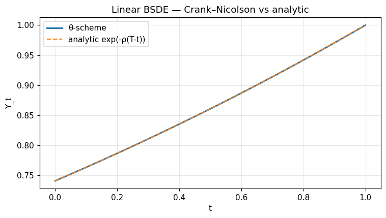
With \(a(t) \equiv -\rho\), \(b = c = 0\) and \(Y_T = 1\) the analytic deterministic solution is \(Y_t = e^{-\rho (T-t)}\).
rho = 0.3
T   = 1.0
res = opt.linear_bsde_constant_coeffs(
    a_const=-rho, b_const=0.0, c_const=0.0,
    terminal=1.0, n_steps=200, t_horizon=T, theta=0.5,
)
tg = np.array(res['time_grid'])
yg = np.array(res['y'])
analytic = np.exp(-rho * (T - tg))
print('Y0 =', yg[0], '   exp(-rho T) =', analytic[0])
print('max abs error =', float(np.max(np.abs(yg - analytic))))
fig, ax = plt.subplots()
ax.plot(tg, yg, label='θ-scheme', lw=2)
ax.plot(tg, analytic, '--', label='analytic exp(-ρ(T-t))')
ax.set_xlabel('t'); ax.set_ylabel('Y_t')
ax.set_title('Linear BSDE — Crank–Nicolson vs analytic')
ax.legend(); ax.grid(alpha=0.3)
fig.tight_layout(); plt.show()

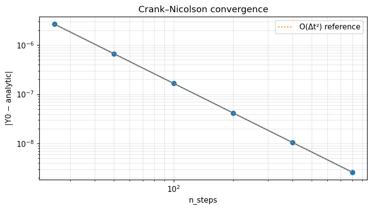
Convergence rate study
Crank–Nicolson is second-order in Δt.
errs = []
ns = [25, 50, 100, 200, 400, 800]
for n in ns:
    r = opt.linear_bsde_constant_coeffs(-rho, 0.0, 0.0, 1.0, n, T, 0.5)
    errs.append(abs(r['y'][0] - np.exp(-rho * T)))
print(list(zip(ns, errs)))
fig, ax = plt.subplots()
ax.loglog(ns, errs, 'o-')
ax.loglog(ns, [errs[0] * (ns[0] / n) ** 2 for n in ns],
          ':', label='O(Δt²) reference')
ax.set_xlabel('n_steps'); ax.set_ylabel('|Y0 − analytic|')
ax.set_title('Crank–Nicolson convergence'); ax.grid(which='both', alpha=0.3); ax.legend()
fig.tight_layout(); plt.show()

Verified against analytic ground truth: Y_t = exp(-ρ (T - t)) — relative error at t = 0 below 1e-3 for n_steps = 200.
API
pub fn solve_linear_bsde<A, B, C>(
    a: A, b: B, c: C, terminal: f64, cfg: &ThetaSchemeConfig
) -> Result<ThetaSchemeResult>
where A: Fn(f64) -> f64, B: Fn(f64) -> f64, C: Fn(f64) -> f64;

pub struct ThetaSchemeConfig { pub n_steps: usize, pub t_horizon: f64, pub theta: f64 }
pub struct ThetaSchemeResult { pub y: Array1<f64>, pub z: Array1<f64>, pub time_grid: Array1<f64> }

pub trait ConditionalExpectation { /* deep-BSDE bridge */ }
pub struct DeepBsdeBridge { /* ... */ }