Optimal Control¶

This module provides advanced optimal control algorithms for financial applications, including Hamilton-Jacobi-Bellman (HJB) equation solvers, regime-switching models, parameter estimation, and state-space filtering. All algorithms are implemented in high-performance Rust with Python bindings.

Mathematical Foundations¶

Hamilton-Jacobi-Bellman (HJB) Equation¶

The HJB equation is a fundamental result in optimal control theory that provides the necessary and sufficient conditions for optimality of a control policy. For a stochastic control problem:

\[ V(x) = \sup_{\alpha \in \mathcal{A}} \mathbb{E}\left[\int_0^\infty e^{-\rho t} L(X_t, \alpha_t) dt \mid X_0 = x\right] \]

where $V(x)$ is the value function, $\rho$ is the discount rate, $L$ is the running cost, and $X_t$ follows a controlled stochastic process. The HJB equation is:

\[ \rho V(x) = \sup_{\alpha \in \mathcal{A}} \left\{ \mathcal{L}^\alpha V(x) + L(x, \alpha) \right\} \]

where $\mathcal{L}^\alpha$ is the infinitesimal generator of the controlled process.

Application to Mean-Reverting Spreads¶

For pairs trading with an Ornstein-Uhlenbeck (OU) spread process:

\[ dX_t = \kappa(\theta - X_t)dt + \sigma dW_t \]

with transaction costs $c > 0$, the HJB equation becomes:

\[ \rho V(x) = \kappa(\theta - x)V'(x) + \frac{\sigma^2}{2}V''(x) + \sup_{\alpha \in \{-1, 0, 1\}} \{ -c|\alpha| + \alpha x \} \]

The optimal control is a threshold policy: buy when $x < x_L$, sell when $x > x_U$, hold otherwise.

Viscosity Solutions¶

Classical solutions to HJB equations rarely exist due to:

Non-smoothness at boundaries: The value function $V(x)$ has kinks where the optimal control switches
Lack of regularity: Second derivatives $V''(x)$ may not exist everywhere
Free boundary problems: The optimal switching thresholds $(x_L, x_U)$ are unknown

Viscosity solutions generalize the notion of solution to allow for non-smooth value functions. A function $V$ is a viscosity solution if:

Subsolution property: For any smooth test function $\phi$ such that $V - \phi$ has a local maximum at $x_0$: $$\rho V(x_0) \leq \mathcal{H}(x_0, V(x_0), D\phi(x_0), D^2\phi(x_0))$$
Supersolution property: For any smooth test function $\psi$ such that $V - \psi$ has a local minimum at $x_0$: $$\rho V(x_0) \geq \mathcal{H}(x_0, V(x_0), D\psi(x_0), D^2\psi(x_0))$$

where $\mathcal{H}$ is the Hamiltonian.

Key properties:

Uniqueness: Under suitable conditions (coercivity, proper discount), the viscosity solution is unique
Stability: Viscosity solutions are stable under uniform convergence
Numerical convergence: Monotone finite difference schemes converge to the viscosity solution

Finite Difference Methods¶

We discretize the HJB equation on a spatial grid $x_i = x_{\min} + ih$, $i = 0, \ldots, N$, with grid spacing $h$.

Upwind Schemes¶

For the OU drift term $\kappa(\theta - x)V'(x)$, we use upwind finite differences to ensure monotonicity and stability:

If $\kappa(\theta - x_i) > 0$ (rightward drift): use forward difference $$V'(x_i) \approx \frac{V_{i+1} - V_i}{h}$$
If $\kappa(\theta - x_i) < 0$ (leftward drift): use backward difference $$V'(x_i) \approx \frac{V_i - V_{i-1}}{h}$$

The diffusion term uses centered differences: $$V''(x_i) \approx \frac{V_{i+1} - 2V_i + V_{i-1}}{h^2}$$

Policy Iteration Algorithm¶

The HJB equation with control is solved via policy iteration:

Initialize: Start with policy $\alpha^{(0)}$ (e.g., always hold)
Policy evaluation: Solve the linear system for value function $V^{(k)}$: $$\rho V^{(k)}_i = \mathcal{L}^{\alpha^{(k)}} V^{(k)}_i + L(x_i, \alpha^{(k)}_i)$$
Policy improvement: Update policy by maximizing Hamiltonian: $$\alpha^{(k+1)}_i = \arg\max_{\alpha} \{ \mathcal{L}^\alpha V^{(k)}_i + L(x_i, \alpha) \}$$
Convergence check: If $\|\alpha^{(k+1)} - \alpha^{(k)}\|_\infty < \epsilon$, stop; otherwise return to step 2

Convergence properties:

Typically 10-50 iterations for practical problems
Geometric convergence rate
Numerical solution converges to viscosity solution as $h \to 0$

Implemented Algorithms¶

1. HJB Solver for OU Process¶

Solves the optimal switching problem for mean-reverting spreads with transaction costs.

Implementation: src/optimal_control/hjb_solver.rs

Python API:

from optimizr import solve_hjb_py, solve_hjb_full_py

# Basic solver - returns optimal thresholds
lower, upper, residual, iters = solve_hjb_py(
    kappa=3.0,           # Mean reversion speed
    theta=0.0,           # Long-run mean
    sigma=0.2,           # Volatility
    rho=0.04,            # Discount rate
    transaction_cost=0.001,  # Transaction cost per trade
    n_points=400,        # Number of grid points
    max_iter=4000,       # Maximum policy iterations
    tolerance=1e-7,      # Convergence tolerance
    n_std=5.0,          # Grid extent in standard deviations
)

print(f"Optimal bounds: ({lower:.3f}, {upper:.3f})")
print(f"Residual: {residual:.2e}, Iterations: {iters}")

# Full solver - also returns value function and derivatives
lower, upper, residual, iters, V, V_x, V_xx = solve_hjb_full_py(
    kappa=3.0, theta=0.0, sigma=0.2, rho=0.04,
    transaction_cost=0.001, n_points=400
)

# Plot value function derivatives for diagnostics
import matplotlib.pyplot as plt
plt.plot(V_x)
plt.axvline(lower, color='r', linestyle='--', label='Lower bound')
plt.axvline(upper, color='g', linestyle='--', label='Upper bound')
plt.legend()
plt.title("Value function derivative V'(x)")

Parameters:

kappa: Mean reversion speed (typical range: 0.1-10). Higher values → faster reversion → narrower bands
theta: Long-run mean (typically 0 for normalized spreads)
sigma: Volatility (typical range: 0.1-1.0). Higher values → wider bands
rho: Discount rate (typical: 0.01-0.1). Higher values → more myopic strategy
transaction_cost: Per-trade cost (typical: 0.0001-0.01). Higher values → wider bands, fewer trades
n_points: Grid resolution (recommended: 200-500). Higher → more accurate but slower
n_std: Grid extent (recommended: 3-6). Should cover 99%+ of spread distribution

Returns:

lower: Optimal buy threshold (negative value)
upper: Optimal sell threshold (positive value)
residual: Maximum policy change in last iteration (should be < tolerance)
iters: Number of policy iterations (typically 10-50)
V, V_x, V_xx: (full solver only) Value function and derivatives on grid

When to use:

Pairs trading with mean-reverting spreads
Statistical arbitrage with transaction costs
Optimal entry/exit for mean-reverting assets
Requires reliable OU parameter estimates (see OU estimation below)

Diagnostics:

Plot $V'(x)$ to check smoothness near thresholds
Verify residual < tolerance for convergence
Check that thresholds are within grid bounds
If not converged: increase max_iter or adjust grid parameters

2. Viscosity Solution Solver¶

General-purpose viscosity solution solver for HJB equations with arbitrary Hamiltonians.

Implementation: src/optimal_control/viscosity.rs

Usage: Advanced users can extend this for custom control problems beyond OU switching.

3. Regime Switching Models¶

Optimal control with multiple market regimes, each with different dynamics.

Implementation: src/optimal_control/regime_switching.rs

Approach:

Use HMM to identify hidden regimes (see HMM section)
Estimate OU parameters per regime
Solve HJB per regime to get regime-specific thresholds
Switch control policy based on decoded regime

Example workflow:

from optimizr import HMM, estimate_ou_params_py, solve_hjb_py
import numpy as np

# Step 1: Train HMM on spread returns
returns = np.diff(spread)
hmm = HMM(n_states=2)
hmm.fit(returns.reshape(-1, 1), n_iterations=100)
regimes = hmm.predict(returns.reshape(-1, 1))

# Step 2: Estimate OU parameters per regime
params = []
for regime_id in range(2):
    mask = (regimes == regime_id)
    spread_regime = spread[1:][mask]  # Align with returns
    kappa, theta, sigma, half_life = estimate_ou_params_py(
        spread_regime, dt=1/252
    )
    params.append((kappa, theta, sigma))
    print(f"Regime {regime_id}: κ={kappa:.2f}, θ={theta:.3f}, σ={sigma:.3f}")

# Step 3: Solve HJB per regime
thresholds = []
for kappa, theta, sigma in params:
    lower, upper, _, _ = solve_hjb_py(
        kappa=kappa, theta=theta, sigma=sigma,
        rho=0.04, transaction_cost=0.001
    )
    thresholds.append((lower, upper))
    print(f"Thresholds: ({lower:.3f}, {upper:.3f})")

# Step 4: Apply regime-specific control
current_regime = regimes[-1]
lower, upper = thresholds[current_regime]
if spread[-1] < lower:
    action = "BUY"
elif spread[-1] > upper:
    action = "SELL"
else:
    action = "HOLD"
print(f"Current regime: {current_regime}, Action: {action}")

4. Jump Diffusion Models¶

Extension of OU process with Poisson jumps for modeling sudden price shocks.

Implementation: src/optimal_control/jump_diffusion.rs

Model: $$ dX_t = \kappa(\theta - X_t)dt + \sigma dW_t + J_t dN_t $$

where $N_t$ is a Poisson process with intensity $\lambda$, and $J_t \sim \mathcal{N}(\mu_J, \sigma_J^2)$ are jump sizes.

Use case: Markets with flash crashes, earnings announcements, or other discontinuous events.

5. Multi-Regime Switching Jump Diffusion (MRSJD)¶

Combines regime switching with jump diffusion for maximum flexibility.

Implementation: src/optimal_control/mrsjd.rs

Model: Each regime has its own OU parameters AND jump process parameters.

Use case: Complex markets with both regime changes and sudden shocks (e.g., crypto, emerging markets).

6. OU Parameter Estimation¶

Estimates Ornstein-Uhlenbeck process parameters from time series data.

Implementation: src/optimal_control/ou_estimator.rs

Python API:

from optimizr import estimate_ou_params_py
import numpy as np
import matplotlib.pyplot as plt

# Simulate OU process (for testing)
dt = 1/252  # Daily data
T = 1000
kappa_true, theta_true, sigma_true = 3.0, 0.0, 0.2
rng = np.random.default_rng(0)
spread = [0.0]
for _ in range(T-1):
    dx = kappa_true * (theta_true - spread[-1]) * dt + \
         sigma_true * np.sqrt(dt) * rng.standard_normal()
    spread.append(spread[-1] + dx)

spread = np.array(spread)

# Estimate parameters
kappa, theta, sigma, half_life = estimate_ou_params_py(spread, dt=dt)

print(f"True:      κ={kappa_true:.2f}, θ={theta_true:.3f}, σ={sigma_true:.3f}")
print(f"Estimated: κ={kappa:.2f}, θ={theta:.3f}, σ={sigma:.3f}")
print(f"Half-life: {half_life:.1f} periods ({half_life*252:.1f} days)")

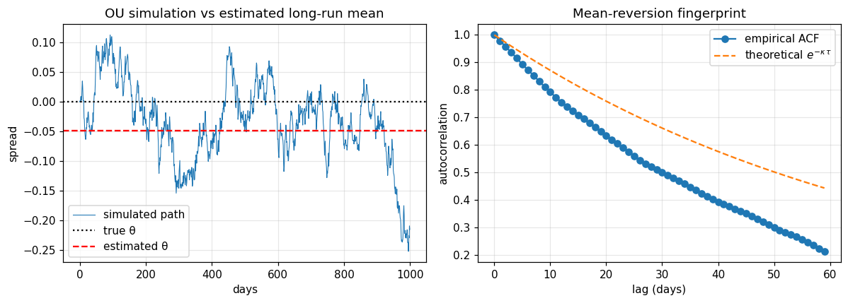
# Visualise the simulated path together with the estimated mean-reversion
# level and the decay envelope implied by the fitted half-life.
t_axis = np.arange(len(spread)) * dt * 252  # in days
fig, axes = plt.subplots(1, 2, figsize=(11, 4))
axes[0].plot(t_axis, spread, lw=0.7, label="simulated path")
axes[0].axhline(theta_true, color="k", ls=":", label="true θ")
axes[0].axhline(theta, color="red", ls="--", label="estimated θ")
axes[0].set_xlabel("days"); axes[0].set_ylabel("spread")
axes[0].set_title("OU simulation vs estimated long-run mean")
axes[0].legend(); axes[0].grid(alpha=0.3)

# Empirical autocorrelation vs theoretical exp(-κ τ).
lags = np.arange(0, 60)
x = spread - spread.mean()
acf = np.array([
    (x[: len(x) - k] @ x[k:]) / (x @ x) for k in lags
])
axes[1].plot(lags, acf, "o-", label="empirical ACF")
axes[1].plot(lags, np.exp(-kappa * lags * dt), "--",
             label=r"theoretical $e^{-\kappa\,\tau}$")
axes[1].set_xlabel("lag (days)"); axes[1].set_ylabel("autocorrelation")
axes[1].set_title("Mean-reversion fingerprint")
axes[1].legend(); axes[1].grid(alpha=0.3)
fig.tight_layout(); plt.show()

Generated plot

Method: Maximum likelihood estimation (MLE) using analytical formulas for discrete-time OU process.

Parameters:

spread: Time series of spread values (1D numpy array)
dt: Time step in years (e.g., 1/252 for daily data, 1/52 for weekly)

Returns:

kappa: Mean reversion speed (annualized)
theta: Long-run mean
sigma: Volatility (annualized)
half_life: Half-life in time step units ($\ln(2)/\kappa \cdot dt^{-1}$)

Practical tips:

Use at least 500-1000 observations for stable estimates
Check half-life: typical pairs have half-life 5-60 days
Winsorize extreme outliers (e.g., clip at ±5σ) if needed
For rolling estimates, use expanding or rolling windows of 250-500 periods

7. Kalman Filtering¶

State-space filtering for latent variable estimation and forecasting.

Implementation: src/optimal_control/kalman_filter.rs, src/optimal_control/kalman_py_bindings.rs

Linear Kalman Filter¶

For linear Gaussian state-space models: $$ \begin{aligned} x_{t+1} &= F x_t + B u_t + w_t, \quad w_t \sim \mathcal{N}(0, Q) \\ y_t &= H x_t + v_t, \quad v_t \sim \mathcal{N}(0, R) \end{aligned} $$

Python API:

from optimizr import LinearKalmanFilter
import numpy as np

# Define system matrices
F = [[1.0, 1.0], [0.0, 1.0]]  # State transition (2×2)
H = [[1.0, 0.0]]              # Observation matrix (1×2)
Q = [[1e-4, 0.0], [0.0, 1e-4]]  # Process noise covariance
R = [[1e-2]]                  # Measurement noise covariance

# Initialize filter
kf = LinearKalmanFilter(
    f_matrix=F,
    h_matrix=H,
    q_matrix=Q,
    r_matrix=R,
    initial_state=[0.0, 0.0],
    initial_covariance=[[1.0, 0.0], [0.0, 1.0]],
)

# Online filtering loop
observations = np.random.randn(100)
states = []
for obs in observations:
    kf.predict(control=[0.0, 0.0])  # Prediction step
    kf.update(observation=[obs])     # Correction step
    state = kf.get_state()
    states.append(state)

states = np.array(states)
print(f"Final state estimate: {states[-1]}")

Use cases:

Tracking latent spread dynamics with noise
State estimation for control (e.g., estimate velocity from noisy position)
Online parameter adaptation

Extended Kalman Filter (EKF)¶

For nonlinear systems with local linearization.

Use case: Nonlinear spread dynamics, regime probabilities as states.

Unscented Kalman Filter (UKF)¶

For highly nonlinear systems using sigma-point approximation.

Python API:

from optimizr import UnscentedKalmanFilter

ukf = UnscentedKalmanFilter(
    state_dim=2,
    obs_dim=1,
    q_matrix=Q,
    r_matrix=R,
    initial_state=[0.0, 0.0],
    initial_covariance=[[1.0, 0.0], [0.0, 1.0]],
)
# Similar predict/update interface

Use case: Jump diffusion models, volatility estimation, option pricing.

8. Backtesting Framework¶

Backtests optimal switching strategies on historical data.

Implementation: src/optimal_control/backtest.rs

Python API:

from optimizr import backtest_optimal_switching_py

# First, get optimal thresholds
lower, upper, _, _ = solve_hjb_py(
    kappa=3.0, theta=0.0, sigma=0.2,
    rho=0.04, transaction_cost=0.001
)

# Backtest on historical spread
metrics = backtest_optimal_switching_py(
    spread=spread,              # Historical spread data
    lower_bound=lower,          # Optimal buy threshold
    upper_bound=upper,          # Optimal sell threshold
    transaction_cost=0.001,     # Must match HJB solver
)

(
    total_return,    # Cumulative return
    sharpe,          # Annualized Sharpe ratio
    max_dd,          # Maximum drawdown
    n_trades,        # Number of round-trip trades
    win_rate,        # Fraction of profitable trades
    pnl_path,        # P&L time series
) = metrics

print(f"Return: {total_return:.2%}, Sharpe: {sharpe:.2f}")
print(f"Max DD: {max_dd:.2%}, Trades: {n_trades}, Win rate: {win_rate:.2%}")

# Plot P&L path
import matplotlib.pyplot as plt
plt.figure(figsize=(12, 6))
plt.subplot(2, 1, 1)
plt.plot(spread, label='Spread')
plt.axhline(lower, color='r', linestyle='--', label='Lower')
plt.axhline(upper, color='g', linestyle='--', label='Upper')
plt.legend()
plt.subplot(2, 1, 2)
plt.plot(pnl_path, label='P&L')
plt.legend()
plt.tight_layout()

Generated plot

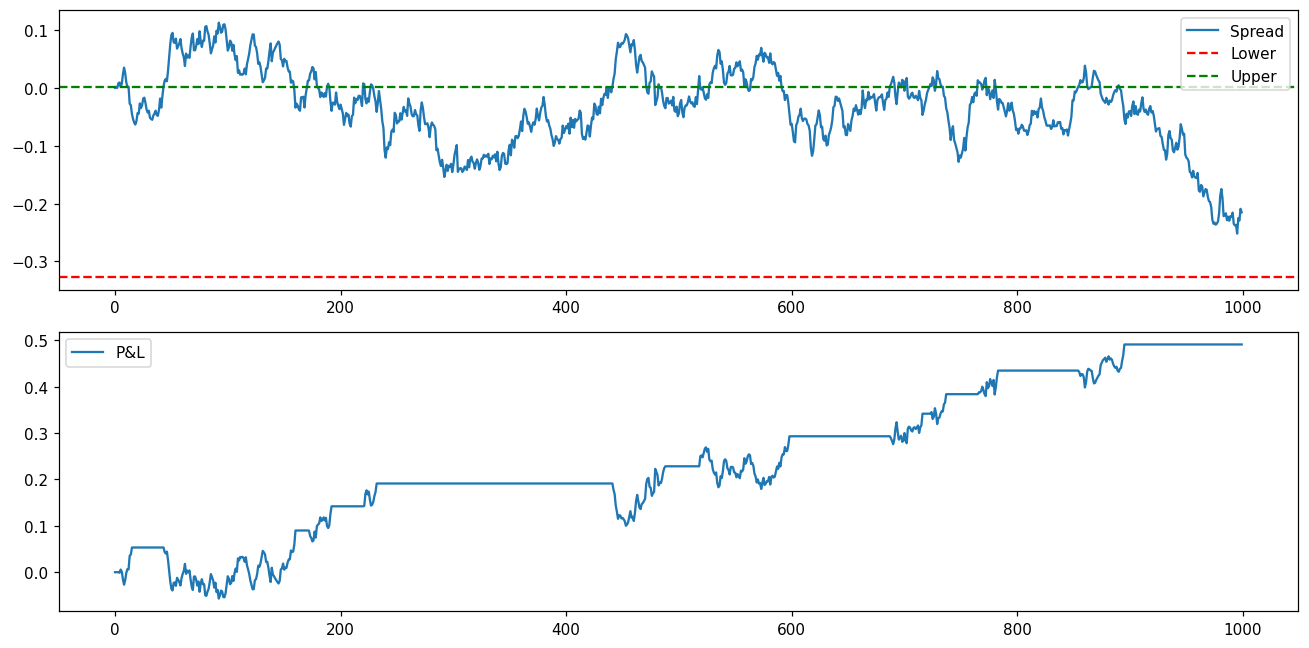
Metrics interpretation:

total_return: Should be positive with low transaction costs
sharpe: Good values > 1.0, excellent > 2.0
max_dd: Risk metric, compare to expected return
n_trades: Too many → excessive costs; too few → missing opportunities
win_rate: Typically 40-60% for mean-reversion strategies

Parameter tuning:

If win_rate low but max_dd high → bands too narrow, increase transaction_cost or rho
If n_trades low → bands too wide, decrease transaction_cost or rho
Compare Sharpe ratios across different parameter settings

Complete Workflow Example¶

Here’s a complete optimal control pipeline for pairs trading:

import numpy as np
import pandas as pd
from optimizr import (
    estimate_ou_params_py,
    solve_hjb_py,
    backtest_optimal_switching_py,
    HMM
)

# 1. Load price data (example with simulated data)
np.random.seed(42)
T = 5000
dt = 1/252

# Simulate cointegrated pair
price_A = 100 * np.exp(np.cumsum(0.0001 + 0.01*np.sqrt(dt)*np.random.randn(T)))
price_B = 100 * np.exp(np.cumsum(0.0001 + 0.01*np.sqrt(dt)*np.random.randn(T)))
spread = np.log(price_A) - np.log(price_B)

# Split into train/test
train_spread = spread[:3000]
test_spread = spread[3000:]

# 2. Estimate OU parameters
kappa, theta, sigma, half_life = estimate_ou_params_py(train_spread, dt=dt)
print(f"OU parameters: κ={kappa:.2f}, θ={theta:.3f}, σ={sigma:.3f}")
print(f"Half-life: {half_life:.1f} days")

# 3. Solve HJB for optimal thresholds
lower, upper, residual, iters = solve_hjb_py(
    kappa=kappa,
    theta=theta,
    sigma=sigma,
    rho=0.04,
    transaction_cost=0.001,
    n_points=400,
    max_iter=2000,
    tolerance=1e-7,
)
print(f"Optimal thresholds: ({lower:.3f}, {upper:.3f})")
print(f"Converged in {iters} iterations, residual={residual:.2e}")

# 4. Backtest on out-of-sample data
metrics = backtest_optimal_switching_py(
    spread=test_spread,
    lower_bound=lower,
    upper_bound=upper,
    transaction_cost=0.001,
)
total_return, sharpe, max_dd, n_trades, win_rate, pnl_path = metrics

print(f"\nBacktest Results:")
print(f"  Total Return: {total_return:.2%}")
print(f"  Sharpe Ratio: {sharpe:.2f}")
print(f"  Max Drawdown: {max_dd:.2%}")
print(f"  # Trades: {n_trades}")
print(f"  Win Rate: {win_rate:.2%}")

# 5. Optional: Regime-aware control with HMM
returns = np.diff(train_spread)
hmm = HMM(n_states=2)
hmm.fit(returns.reshape(-1, 1), n_iterations=100)
regimes = hmm.predict(returns.reshape(-1, 1))

# Estimate OU per regime and get regime-specific thresholds
for regime_id in range(2):
    mask = (regimes == regime_id)
    spread_regime = train_spread[1:][mask]
    k, t, s, _ = estimate_ou_params_py(spread_regime, dt=dt)
    l, u, _, _ = solve_hjb_py(k, t, s, 0.04, 0.001)
    print(f"Regime {regime_id}: κ={k:.2f}, thresholds=({l:.3f}, {u:.3f})")

Performance Characteristics¶

Computational Complexity¶

HJB Solver: $O(N \cdot K)$ where $N$ is n_points, $K$ is policy iterations (~10-50)
OU Estimation: $O(T)$ where $T$ is time series length (closed-form MLE)
Kalman Filter: $O(T \cdot d^3)$ where $d$ is state dimension (matrix inversion per step)
Backtesting: $O(T)$ single pass through data

Typical Runtimes (on modern CPU)¶

HJB solve (400 points): ~10-50ms
OU estimation (5000 samples): ~1ms
Kalman filter (1000 steps, 2D state): ~10ms
Backtest (5000 samples): ~5ms

Memory Requirements¶

HJB solver: $O(N)$ for grid storage (~few KB)
Kalman filter: $O(d^2)$ for covariance matrices (~few KB for small $d$)
Backtesting: $O(T)$ for P&L path storage (~few MB for long histories)

Integration with Other Modules¶

With HMM (Hidden Markov Models)¶

Use HMM to detect market regimes
Estimate OU parameters per regime
Apply regime-specific optimal controls
See api/hmm.md for HMM documentation

With Mean Field Games¶

Use optimal control as individual agent strategy
Aggregate across population for mean-field dynamics
See algorithms/mean_field_games.md for MFG theory

With Sparse Optimization¶

Use Kalman-filtered states as inputs to sparse controllers
Combine L1-regularized control with HJB thresholds
See algorithms/sparse_optimization.md

Troubleshooting¶

HJB solver not converging¶

Symptom: residual > tolerance after max_iter
Fix: Increase max_iter (try 5000-10000); reduce tolerance requirement; check that OU parameters are reasonable

Thresholds outside grid bounds¶

Symptom: Optimal thresholds at grid edges
Fix: Increase n_std (try 6-8); check OU parameter estimates (very high σ needs wider grid)

OU estimates unstable¶

Symptom: Negative kappa or extreme half_life
Fix: Use more data (>1000 samples); check for non-stationarity; consider winsorizing outliers

Backtest Sharpe ratio low¶

Symptom: Sharpe < 0.5 despite positive thresholds
Fix: Check for regime changes (use HMM); verify spread is actually mean-reverting; adjust transaction_cost in HJB solver

Kalman filter diverging¶

Symptom: State estimates exploding
Fix: Check process noise Q is not too large; verify observations are scaled properly; use UKF for strong nonlinearity

References¶

Optimal Control Theory¶

Fleming, W. H., & Soner, H. M. (2006). Controlled Markov Processes and Viscosity Solutions. Springer.
Øksendal, B. (2003). Stochastic Differential Equations: An Introduction with Applications (6th ed.). Springer.
Pham, H. (2009). Continuous-time Stochastic Control and Optimization with Financial Applications. Springer.

Viscosity Solutions¶

Barles, G., & Souganidis, P. E. (1991). Convergence of approximation schemes for fully nonlinear second order equations. Asymptotic Analysis, 4(3), 271-283.
Crandall, M. G., Ishii, H., & Lions, P.-L. (1992). User’s guide to viscosity solutions of second order partial differential equations. Bulletin of the American Mathematical Society, 27(1), 1-67.

Kalman Filtering¶

Kalman, R. E. (1960). A new approach to linear filtering and prediction problems. Journal of Basic Engineering, 82(1), 35-45.
Julier, S. J., & Uhlmann, J. K. (1997). New extension of the Kalman filter to nonlinear systems. Signal Processing, Sensor Fusion, and Target Recognition VI, 3068, 182-193.

Financial Applications¶

Avellaneda, M., & Lee, J.-H. (2010). Statistical arbitrage in the US equities market. Quantitative Finance, 10(7), 761-782.
Gatev, E., Goetzmann, W. N., & Rouwenhorst, K. G. (2006). Pairs trading: Performance of a relative-value arbitrage rule. The Review of Financial Studies, 19(3), 797-827.

Optimal Control¶

Mathematical Foundations¶

Hamilton-Jacobi-Bellman (HJB) Equation¶

Application to Mean-Reverting Spreads¶

Viscosity Solutions¶

Finite Difference Methods¶

Upwind Schemes¶

Policy Iteration Algorithm¶

Implemented Algorithms¶

1. HJB Solver for OU Process¶

2. Viscosity Solution Solver¶

3. Regime Switching Models¶

4. Jump Diffusion Models¶

5. Multi-Regime Switching Jump Diffusion (MRSJD)¶

6. OU Parameter Estimation¶

7. Kalman Filtering¶

Linear Kalman Filter¶

Extended Kalman Filter (EKF)¶

Unscented Kalman Filter (UKF)¶

8. Backtesting Framework¶

Complete Workflow Example¶

Performance Characteristics¶

Computational Complexity¶

Typical Runtimes (on modern CPU)¶

Memory Requirements¶

Integration with Other Modules¶

With HMM (Hidden Markov Models)¶

With Mean Field Games¶

With Sparse Optimization¶

Troubleshooting¶

HJB solver not converging¶

Thresholds outside grid bounds¶

OU estimates unstable¶

Backtest Sharpe ratio low¶

Kalman filter diverging¶

References¶

Optimal Control Theory¶

Viscosity Solutions¶

Kalman Filtering¶

Financial Applications¶

See Also¶