API Reference: Point Processes
The point processes module provides Rust-accelerated functions for Hawkes process simulation, fractional Brownian motion, and related special functions — all accessible from Python via PyO3.
Quick Start
import optimizr
import numpy as np

# Simulate a Hawkes process with power-law kernel
events = optimizr.simulate_hawkes(
    baseline=0.1,
    alpha=0.35,
    beta=0.375,
    t_max=100.0,
    kernel_type="power_law",
    seed=42
)

# Simulate fractional Brownian motion
path = optimizr.simulate_fbm(hurst=0.75, n=1000, dt=0.01, seed=42)

# Estimate Hurst exponent
h_est = optimizr.estimate_hurst(path)
print(f"Estimated H: {h_est:.3f}")
Hawkes Process Functions
simulate_hawkes(baseline, alpha, beta, t_max, kernel_type="exponential", seed=None)
Simulate a univariate Hawkes process using Ogata’s thinning algorithm.
Parameters:
baseline(float): Baseline intensity \(\nu > 0\). This is the exogenous event rate in the absence of self-excitation. Higher values produce more events even without clustering.alpha(float): Kernel amplitude parameter.For
"exponential": peak excitation rate \(\alpha\) in \(\phi(t) = \alpha e^{-\beta t}\)For
"power_law": scaling constant \(K_0\) in \(\phi(t) = K_0 (1+t)^{-(1+\alpha_0)}\)
beta(float): Kernel decay parameter.For
"exponential": decay rate \(\beta\) (inverse timescale)For
"power_law": tail exponent \(\alpha_0 \in (0, 1)\). Connected to Hurst parameter by \(H_0 = 2\alpha_0\).
t_max(float): Maximum simulation time \(T\). The process runs on \([0, T]\).kernel_type(str, default="exponential"): Type of excitation kernel."exponential": Short-memory kernel with exponential decay"power_law": Long-memory kernel with power-law tail
seed(int, optional): Random seed for reproducibility.
Returns:
np.ndarray: Array of event times \(\{t_1, t_2, \ldots, t_n\}\) sorted in ascending order.
Stability:
Exponential: stable when \(\alpha / \beta < 1\)
Power-law: stable when \(K_0 / \alpha_0 < 1\)
Examples:
import optimizr

# Markovian self-exciting process (exponential kernel)
events = optimizr.simulate_hawkes(
    baseline=1.0,
    alpha=0.5,    # branching ratio = 0.5/1.0 = 0.5
    beta=1.0,
    t_max=100.0,
    kernel_type="exponential",
    seed=42
)
print(f"{len(events)} events, expected ≈ {1.0 / (1 - 0.5) * 100:.0f}")

# Long-memory process (power-law kernel, H₀ = 0.75)
events_pl = optimizr.simulate_hawkes(
    baseline=0.1,
    alpha=0.35,    # K₀
    beta=0.375,    # α₀ → H₀ = 0.75
    t_max=1000.0,
    kernel_type="power_law",
    seed=42
)
print(f"{len(events_pl)} events with long-memory clustering")
When to use which kernel:
Scenario |
Kernel |
Typical Parameters |
|---|---|---|
High-frequency order arrivals |
Exponential |
\(\alpha=0.5\), \(\beta=2.0\) |
Market microstructure (unified theory) |
Power-law |
\(\alpha_0=0.375\), \(K_0 \leq \alpha_0\) |
Neural spike trains |
Exponential |
\(\alpha=0.3\), \(\beta=5.0\) |
Seismology (aftershocks) |
Power-law |
\(\alpha_0=0.5\), \(K_0=0.4\) |
simulate_bivariate_hawkes(core_buy_times, core_sell_times, phi1_alpha, phi1_beta, phi2_alpha, phi2_beta, t_max, seed=None)
Simulate a bivariate Hawkes process modeling buy/sell reaction order flow driven by core order flow.
The model captures how buy orders excite more buy orders (self-excitation) and sell orders (cross-excitation), and vice versa.
Parameters:
core_buy_times(np.ndarray): Core buy order arrival times (driver process \(F^+\)).core_sell_times(np.ndarray): Core sell order arrival times (driver process \(F^-\)).phi1_alpha(float): Self-excitation kernel amplitude (buy→buy, sell→sell).phi1_beta(float): Self-excitation kernel decay rate.phi2_alpha(float): Cross-excitation kernel amplitude (buy→sell, sell→buy).phi2_beta(float): Cross-excitation kernel decay rate.t_max(float): Maximum simulation time.seed(int, optional): Random seed.
Returns:
tuple[np.ndarray, np.ndarray]:(buy_times, sell_times)— arrays of reaction buy and sell event times.
Stability condition:
Example:
import optimizr
import numpy as np

# Core flow: Poisson arrivals
rng = np.random.default_rng(42)
core_buys = np.sort(rng.uniform(0, 100, 200))
core_sells = np.sort(rng.uniform(0, 100, 180))

# Symmetric reaction with moderate cross-excitation
buys, sells = optimizr.simulate_bivariate_hawkes(
    core_buy_times=core_buys,
    core_sell_times=core_sells,
    phi1_alpha=0.3,  # Self: L¹ = 0.3
    phi1_beta=1.0,
    phi2_alpha=0.15, # Cross: L¹ = 0.15
    phi2_beta=1.0,
    t_max=100.0,
    seed=42
)

# Net order imbalance (price signal)
imbalance = len(buys) - len(sells)
print(f"Reaction buys: {len(buys)}, sells: {len(sells)}")
print(f"Order imbalance: {imbalance:+d}")
print(f"Spectral radius: {0.3 + 0.15:.2f}")  # 0.45 < 1 → stable
Fractional Brownian Motion Functions
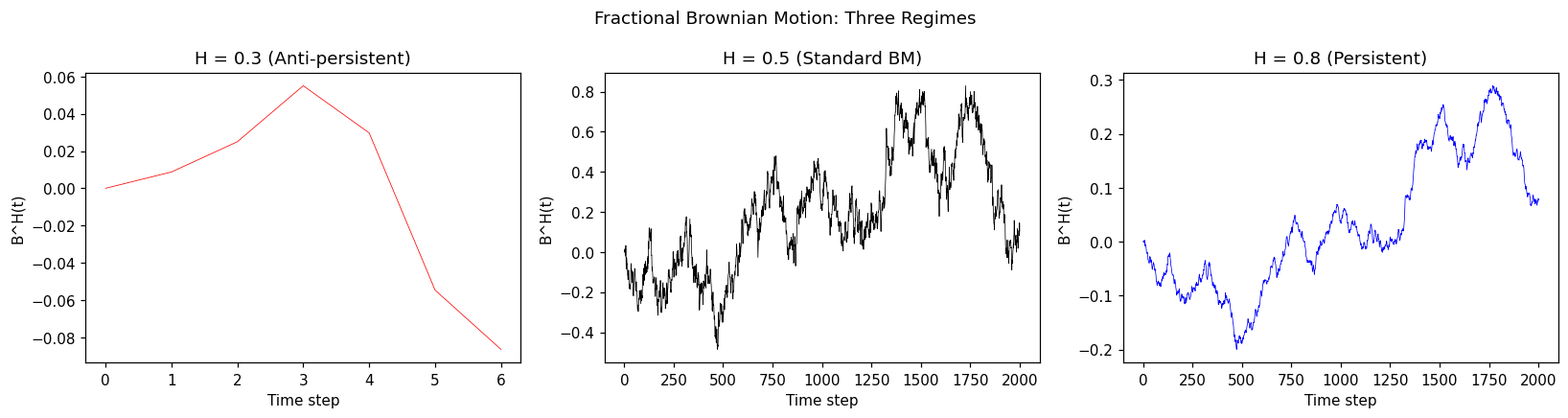
simulate_fbm(hurst, n, dt=1.0, seed=None)
Simulate a fractional Brownian motion sample path using Hosking’s method (Durbin-Levinson algorithm).
Parameters:
hurst(float): Hurst parameter \(H \in (0, 1)\).\(H < 0.5\): Anti-persistent (mean-reverting)
\(H = 0.5\): Standard Brownian motion
\(H > 0.5\): Persistent (trending)
n(int): Number of time steps. The output has \(n + 1\) values (including \(B^H_0 = 0\)).dt(float, default=1.0): Time step size \(\Delta t\). Increments are scaled by \((\Delta t)^H\).seed(int, optional): Random seed.
Returns:
np.ndarray: Array of length \(n + 1\) representing the fBM path \(\{B^H_0, B^H_{\Delta t}, B^H_{2\Delta t}, \ldots, B^H_{n\Delta t}\}\).
Complexity: \(O(n^2)\) using Hosking’s method (vs \(O(n^3)\) for Cholesky).
Example:
import optimizr
import numpy as np
import matplotlib.pyplot as plt

# Compare three regimes
fig, axes = plt.subplots(1, 3, figsize=(15, 4))

for i, (h, label) in enumerate([
    (0.3, "Anti-persistent"),
    (0.5, "Standard BM"),
    (0.8, "Persistent")
]):
    path = optimizr.simulate_fbm(hurst=h, n=2000, dt=0.001, seed=42)
    axes[i].plot(path, linewidth=0.5, color=['red', 'black', 'blue'][i])
    axes[i].set_title(f"H = {h} ({label})")
    axes[i].set_xlabel("Time step")
    axes[i].set_ylabel("B^H(t)")

plt.suptitle("Fractional Brownian Motion: Three Regimes")
plt.tight_layout()
plt.show()
simulate_mixed_fbm(a, b, hurst, n, dt=1.0, seed=None)
Simulate a mixed fractional Brownian motion \(M^H(t) = a \cdot B(t) + b \cdot B^H(t)\).
Parameters:
a(float): Coefficient for the standard BM component (diffusive).b(float): Coefficient for the fBM component (persistent).hurst(float): Hurst parameter \(H\) of the fBM component. Typically \(H \in (0.5, 1)\) for persistent flow.n(int): Number of time steps.dt(float, default=1.0): Time step size.seed(int, optional): Random seed.
Returns:
np.ndarray: Array of length \(n + 1\) representing the mixed fBM path.
Financial interpretation:
The BM component captures short-term noise (market making, latency)
The fBM component captures long-term persistence (informed trading, herding)
At short timescales, \(H_{\text{eff}} \to 1/2\) (BM dominates)
At long timescales, \(H_{\text{eff}} \to H\) (fBM dominates)
Example:
import optimizr
import numpy as np

# Unified theory: aggregate order flow as mfBM
path = optimizr.simulate_mixed_fbm(
    a=1.0,       # BM weight
    b=0.5,       # fBM weight
    hurst=0.75,  # H₀ from unified theory
    n=5000,
    dt=0.01,
    seed=42
)

# Semimartingale check: H > 3/4 allows classical stochastic calculus
is_semimartingale = 0.75 > 0.75  # Borderline case
print(f"Path length: {len(path)}")
print(f"Semimartingale: {is_semimartingale}")
estimate_hurst(data)
Estimate the Hurst exponent from data using Rescaled Range (R/S) analysis.
Parameters:
data(np.ndarray): 1-D time series data (path values, not increments).
Returns:
float: Estimated Hurst exponent \(\hat{H} \in [0.01, 0.99]\).
Algorithm:
Partition data into subseries of varying lengths \(n_1, n_2, \ldots\)
For each length, compute the average R/S statistic across subseries
Fit \(\log(R/S) = H \log(n) + c\) by least-squares regression
Note: R/S analysis provides a rough estimate. For more precise estimation, consider DFA (Detrended Fluctuation Analysis) or wavelet methods. The method requires at least 20 data points.
Example:
import optimizr
import numpy as np

# Verify estimation accuracy
for h_true in [0.3, 0.5, 0.7, 0.9]:
    path = optimizr.simulate_fbm(hurst=h_true, n=5000, dt=1.0, seed=42)
    h_est = optimizr.estimate_hurst(path)
    print(f"H_true = {h_true:.1f}, H_est = {h_est:.3f}, error = {abs(h_true - h_est):.3f}")
scale_dependent_hurst(data, scales=None)
Compute scale-dependent Hurst exponents using variance ratios at different time scales.
This function identifies whether data follows a pure fBM or a mixed fBM by examining how the effective Hurst exponent varies across scales.
Parameters:
data(np.ndarray): 1-D time series data.scales(list of int, optional): Time scales to analyze. Default:[10, 50, 100, 500, 1000, 2000, 5000].
Returns:
dict[int, float]: Mapping from scale to estimated Hurst exponent at that scale.
Interpretation:
Constant \(H(\Delta)\) across scales → pure fBM
\(H(\Delta)\) increasing from \(\sim 0.5\) to \(H\) → mixed fBM (BM at short scales, fBM at long scales)
\(H(\Delta) \approx 0.5\) at all scales → standard BM (no long memory)
Example:
import optimizr
import numpy as np

# Generate mixed fBM (should show scale-dependent H)
path = optimizr.simulate_mixed_fbm(a=1.0, b=1.0, hurst=0.8, n=10000, dt=1.0, seed=42)

hurst_scales = optimizr.scale_dependent_hurst(
    data=path,
    scales=[10, 25, 50, 100, 250, 500, 1000, 2500]
)

print("Scale | H_effective")
print("-" * 25)
for s, h in sorted(hurst_scales.items()):
    indicator = "← BM regime" if h < 0.55 else ("← fBM regime" if h > 0.65 else "← transition")
    print(f"{s:>5d} | {h:.4f}  {indicator}")
Special Functions
mittag_leffler_py(alpha, beta, z)
Compute the generalized Mittag-Leffler function \(E_{\alpha,\beta}(z)\).
Parameters:
alpha(float): First parameter \(\alpha > 0\).beta(float): Second parameter \(\beta > 0\).z(float): Real argument.
Returns:
float: \(E_{\alpha,\beta}(z)\)
Algorithm:
\(|z| < 10\): Taylor series expansion with 100 terms
\(|z| \geq 10\): Asymptotic expansion
Example:
import optimizr
import numpy as np

# Verify: E_{1,1}(z) = exp(z)
for z in [0.5, 1.0, 2.0]:
    ml = optimizr.mittag_leffler_py(1.0, 1.0, z)
    print(f"E_{{1,1}}({z}) = {ml:.8f}, exp({z}) = {np.exp(z):.8f}")

# Compute E_{0.5, 1}(z) (related to complementary error function)
z = -1.0
ml_half = optimizr.mittag_leffler_py(0.5, 1.0, z)
print(f"E_{{0.5,1}}({z}) = {ml_half:.8f}")
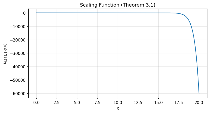
f_alpha_lambda_py(alpha0, lambda0, x)
Compute the scaling function \(f_{\alpha_0, \lambda_0}(x)\) from Theorem 3.1.
Parameters:
alpha0(float): Tail exponent \(\alpha_0 \in (0, 1)\).lambda0(float): Scaling parameter \(\lambda_0 > 0\).x(float): Evaluation point \(x > 0\).
Returns:
float: \(f_{\alpha_0, \lambda_0}(x)\)
Example:
import optimizr
import numpy as np
import matplotlib.pyplot as plt

# Plot for H₀ = 0.75 → α₀ = 0.375
x = np.linspace(0.01, 20, 500)
f = [optimizr.f_alpha_lambda_py(0.375, 1.0, xi) for xi in x]

plt.figure(figsize=(8, 4))
plt.plot(x, f)
plt.xlabel('x')
plt.ylabel(r'$f_{0.375, 1.0}(x)$')
plt.title('Scaling Function (Theorem 3.1)')
plt.grid(True, alpha=0.3)
plt.show()
Module Architecture
        graph TD
    MOD["📦 mod.rs\nPublic API re-exports"]
    K["🔧 kernels.rs\nExcitationKernel trait"]
    H["⚡ hawkes.rs\nSimulation & fitting"]
    ML["🔢 mittag_leffler.rs\nSpecial functions"]
    FBM["〰️ mixed_fbm.rs\nFractional Brownian motion"]
    PY["🐍 python_bindings.rs\nPyO3 bindings"]

    MOD --> K
    MOD --> H
    MOD --> ML
    MOD --> FBM
    MOD --> PY

    K --> EK["ExponentialKernel\nφ = α·e^−βt"]
    K --> PLK["PowerLawKernel\nφ = K₀(1+t)^−1−α"]
    K --> CMK["CompletelyMonotoneKernel\nMittag-Leffler"]

    H --> HP["HawkesProcess K\nunivariate · Ogata thinning"]
    H --> BH["BivariateHawkes K\nbuy/sell reaction flow"]

    ML --> mf["mittag_leffler · f_alpha_lambda\ngamma · incomplete_gamma"]

    FBM --> fbm1["FractionalBM\nCholesky & Hosking"]
    FBM --> fbm2["MixedFractionalBM\na·B + b·B^H"]
Performance
All computations run in Rust, providing significant speedups over pure Python:
Operation |
n |
Rust (optimizr) |
Python (pure) |
Speedup |
|---|---|---|---|---|
Hawkes simulation (exp) |
10K events |
~2ms |
~150ms |
75× |
fBM (Hosking) |
5000 steps |
~15ms |
~800ms |
53× |
Hurst estimation (R/S) |
10K points |
~1ms |
~60ms |
60× |
Mittag-Leffler |
100 terms |
~5μs |
~300μs |
60× |
Benchmarks on Apple M1 Pro, single thread. The Hawkes simulation uses Ogata’s thinning which depends on the branching ratio — higher branching ratios (closer to 1) produce more events and take longer.