Point Processes & Fractional Brownian Motion¶

This module implements the mathematical framework from Muhle-Karbe, Jusselin & Rosenbaum (2022) for modeling order flow microstructure through self-exciting point processes and fractional dynamics.

It provides high-performance Rust implementations of:

Hawkes Processes with flexible excitation kernels
Fractional Brownian Motion (fBM) with exact simulation
Mixed Fractional Brownian Motion (mfBM) for aggregate flow
Mittag-Leffler Functions for scaling limit analysis

Mathematical Foundations¶

The Unified Theory of Order Flow¶

The key insight from the unified theory is that a single parameter — the Hurst exponent \(H_0 \approx 3/4\) — governs all market microstructure quantities:

\[ \boxed{H_0 \approx \frac{3}{4}} \]

This parameter determines:

Quantity	Formula	Value at \(H_0 = 3/4\)
Price roughness	\(H_{\text{price}} = H_0 - \tfrac{1}{2}\)	\(1/4\)
Volatility roughness	\(H_{\text{vol}} \approx H_0 - \tfrac{1}{2}\)	\(\approx 0.1\)
Market impact exponent	\(\delta = 1 - \tfrac{1}{2H_0}\)	\(1/3\)
Kyle’s lambda	\(\Lambda \sim n^{-\delta}\)	\(\sim n^{-1/3}\)
Kernel tail exponent	\(\alpha_0 = H_0/2\)	\(3/8\)

The model structure is:

\[ N = F + R \]

where:

\(N\) = total order flow (observable)
\(F\) = core (fundamental) order flow
\(R\) = reaction (self-exciting) order flow modeled by Hawkes processes

Hawkes Processes¶

Definition¶

A (univariate) Hawkes process \(N(t)\) has conditional intensity:

\[ \lambda(t) = \nu + \int_0^{t^-} \phi(t - s) \, dN(s) = \nu + \sum_{t_i < t} \phi(t - t_i) \]

where:

\(\nu > 0\) is the baseline intensity (exogenous arrival rate)
\(\phi: \mathbb{R}_+ \to \mathbb{R}_+\) is the excitation kernel (self-exciting memory)
\(t_i\) are past event times

The process is stable (stationary) when the branching ratio satisfies:

\[ \|\phi\|_{L^1} = \int_0^\infty \phi(t) \, dt < 1 \]

The expected number of events per unit time in stationarity is:

\[ \mathbb{E}[\lambda] = \frac{\nu}{1 - \|\phi\|_{L^1}} \]

Excitation Kernels¶

Exponential Kernel (Short Memory)¶

\[ \phi(t) = \alpha \, e^{-\beta t}, \quad \alpha, \beta > 0 \]

Properties:

L¹ norm: \(\|\phi\|_{L^1} = \alpha / \beta\)
Stability: \(\alpha < \beta\)
Half-life: \(t_{1/2} = \ln 2 / \beta\)
Tail: exponential decay (no long memory)
Characteristic timescale: \(\tau = 1/\beta\)

The exponential kernel leads to an intensity process that is Markovian — the full history can be summarized by the current intensity level. The integrated kernel is:

\[ \int_0^t \phi(s) \, ds = \frac{\alpha}{\beta} \left(1 - e^{-\beta t}\right) \]

Power-Law Kernel (Long Memory)¶

\[ \phi(t) = K_0 \, (1 + t)^{-(1 + \alpha_0)}, \quad K_0 > 0, \; \alpha_0 \in (0, 1) \]

Properties:

L¹ norm: \(\|\phi\|_{L^1} = K_0 / \alpha_0\)
Stability: \(K_0 < \alpha_0\)
Tail exponent: \(\alpha_0\) controls memory persistence
Hurst connection: \(H_0 = 2\alpha_0\) (from the unified theory)
Long memory: polynomial decay produces clustering at all timescales

The integrated kernel is:

\[ \int_0^t \phi(s) \, ds = \frac{K_0}{\alpha_0} \left[1 - (1 + t)^{-\alpha_0}\right] \]

The critical regime (\(\|\phi\|_{L^1} = 1\)) corresponds to \(K_0 = \alpha_0\), and the nearly-critical regime (\(\|\phi\|_{L^1} = 1 - \varepsilon\)) is relevant for real market data where the branching ratio is very close to 1.

Completely Monotone Kernel (Assumption A)¶

From the unified theory paper’s Assumption A, the most general kernel satisfying the scaling limit theorems:

\[ \phi(t) = K_0 \, t^{-\alpha_0} \, E_{1-\alpha_0}\!\left(-\lambda \, t^{1-\alpha_0}\right) \]

where \(E_\alpha\) is the Mittag-Leffler function. This kernel:

Is completely monotone on \((0, \infty)\)
Interpolates between power-law and exponential behavior
Satisfies all conditions for the scaling limit theorems

Simulation: Ogata’s Thinning Algorithm¶

The Hawkes process is simulated using Ogata’s thinning algorithm:

Compute upper bound \(\lambda_{\max} \geq \lambda(t)\) for the current intensity
Generate candidate inter-arrival time \(\tau \sim \text{Exp}(\lambda_{\max})\)
Accept with probability \(\lambda(t + \tau) / \lambda_{\max}\)
If rejected, advance time to \(t + \tau\) and repeat

The algorithm has expected time complexity \(O(n \log n)\) where \(n\) is the number of events.

Maximum Likelihood Estimation¶

The log-likelihood of a Hawkes process on \([0, T]\) with event times \(\{t_1, \ldots, t_n\}\):

\[ \ell(\boldsymbol{\theta}) = \sum_{i=1}^n \log \lambda(t_i) - \int_0^T \lambda(t) \, dt \]

The compensator (integrated intensity) decomposes as:

\[ \int_0^T \lambda(t) \, dt = \nu T + \sum_{i=1}^n \int_0^{T - t_i} \phi(s) \, ds \]

Bivariate Hawkes Process¶

For order flow modeling, buy and sell reaction orders follow a bivariate Hawkes process \(\mathbf{N} = (N^+, N^-)\) with intensity:

\[\begin{split} \begin{aligned} \lambda^+(t) &= \mu^+(t) + \int \left[\phi_1(t-s) \, dN^+(s) + \phi_2(t-s) \, dN^-(s)\right] \\ \lambda^-(t) &= \mu^-(t) + \int \left[\phi_2(t-s) \, dN^+(s) + \phi_1(t-s) \, dN^-(s)\right] \end{aligned} \end{split}\]

where:

\(\phi_1\): self-excitation kernel (buy \(\to\) buy, sell \(\to\) sell)
\(\phi_2\): cross-excitation kernel (buy \(\to\) sell, sell \(\to\) buy)
\(\mu^\pm(t)\): baselines driven by core order flow

The stability condition requires the spectral radius of the kernel matrix:

\[\begin{split} \rho\!\left(\begin{pmatrix} \|\phi_1\|_1 & \|\phi_2\|_1 \\ \|\phi_2\|_1 & \|\phi_1\|_1 \end{pmatrix}\right) = \|\phi_1\|_1 + \|\phi_2\|_1 < 1 \end{split}\]

The signed flow \(N^+(t) - N^-(t)\) captures the net order imbalance driving price changes, while the unsigned volume \(N^+(t) + N^-(t)\) measures total reaction activity.

Fractional Brownian Motion¶

Definition¶

Fractional Brownian motion (fBM) \(B^H_t\) with Hurst parameter \(H \in (0, 1)\) is the unique centered Gaussian process with:

\[ \text{Cov}(B^H_s, B^H_t) = \frac{1}{2}\left(|t|^{2H} + |s|^{2H} - |t-s|^{2H}\right) \]

Key properties:

Self-similarity: \(B^H_{ct} \overset{d}{=} c^H B^H_t\) for all \(c > 0\)
Stationary increments: \(B^H_t - B^H_s \overset{d}{=} B^H_{t-s}\)
Variance: \(\text{Var}(B^H_t) = t^{2H}\)

The three regimes are:

Range	Behavior	Autocorrelation	Financial Interpretation
\(H < 1/2\)	Anti-persistent (mean-reverting)	Negative	Price reversals dominate
\(H = 1/2\)	Standard BM (no memory)	Zero	Random walk
\(H > 1/2\)	Persistent (trending)	Positive	Trends persist

Fractional Gaussian Noise (fGn)¶

The increments of fBM form fractional Gaussian noise with autocovariance:

\[ \gamma(k) = \frac{1}{2}\left(|k-1|^{2H} - 2|k|^{2H} + |k+1|^{2H}\right) \]

For \(H > 1/2\), \(\gamma(k) > 0\) for all \(k\), indicating long-range dependence:

\[ \sum_{k=0}^\infty \gamma(k) = \infty \]

Simulation Methods¶

Cholesky Method¶

Exact simulation by forming the covariance matrix \(\Sigma\) and computing its Cholesky decomposition:

\[ \Sigma = L L^\top, \quad \mathbf{B}^H = L \mathbf{Z}, \quad \mathbf{Z} \sim \mathcal{N}(\mathbf{0}, I_n) \]

Complexity: \(O(n^3)\) for decomposition, \(O(n^2)\) for simulation.

Hosking’s Method (Durbin-Levinson)¶

For regular time grids, uses the Durbin-Levinson algorithm to compute prediction coefficients for the fGn, then reconstructs fBM by cumulative summation:

Compute autocovariance sequence \(\gamma(0), \gamma(1), \ldots, \gamma(n-1)\)
Recursively compute Levinson coefficients \(\phi_{i,j}\) and prediction variances \(v_i\)
Generate fGn: \(X_i = \sum_{j=0}^{i-1} \phi_{i,j} X_{i-1-j} + \sqrt{v_i} Z_i\)
Cumulate: \(B^H_k = \sum_{i=0}^{k-1} X_i \cdot (\Delta t)^H\)

Complexity: \(O(n^2)\) — more efficient than Cholesky for large \(n\).

Hurst Exponent Estimation¶

Rescaled Range (R/S) Analysis¶

The R/S statistic for a subseries of length \(n\):

\[ (R/S)_n = \frac{\max_{1 \leq k \leq n} W_k - \min_{1 \leq k \leq n} W_k}{S_n} \]

where \(W_k = \sum_{i=1}^k (X_i - \bar{X})\) is the cumulative deviation and \(S_n\) is the standard deviation.

For fBM/fGn:

\[ \mathbb{E}[(R/S)_n] \sim c \cdot n^H \quad \text{as } n \to \infty \]

The Hurst exponent is estimated by linear regression of \(\log(R/S)\) against \(\log n\):

\[ \hat{H} = \frac{\sum_i (\log n_i - \overline{\log n})(\log(R/S)_i - \overline{\log(R/S)})}{\sum_i (\log n_i - \overline{\log n})^2} \]

Mixed Fractional Brownian Motion¶

Definition¶

The mixed fBM (mfBM) combines a standard BM with an independent fBM:

\[ M^H(t) = a \cdot B(t) + b \cdot B^H(t) \]

where:

\(B(t)\): standard Brownian motion (diffusive component)
\(B^H(t)\): fractional BM with Hurst index \(H\)
\(a, b\): mixing coefficients

Covariance Structure¶

\[ \text{Cov}(M^H_s, M^H_t) = a^2 \min(s,t) + \frac{b^2}{2}\left(|t|^{2H} + |s|^{2H} - |t-s|^{2H}\right) \]

Role in the Unified Theory¶

In the scaling limit of the Hawkes-based order flow model, the aggregate order flow converges to:

\[ \frac{1}{\sqrt{n}} \sum_{i=1}^{\lfloor nt \rfloor} (N^+_i - N^-_i) \xrightarrow{d} \sigma_F \cdot M^{H_0}(t) \]

where the Hurst exponent \(H_0 = 2\alpha_0\) is determined by the kernel tail.

Semimartingale Property¶

The mfBM is a semimartingale if and only if \(H > 3/4\). This has pricing implications:

For \(H > 3/4\): classical stochastic calculus applies, no arbitrage
For \(H \leq 3/4\): not a semimartingale, requires fractional calculus

Scale-Dependent Hurst Analysis¶

To identify a mfBM (vs pure fBM or BM), examine the scale-dependent Hurst exponent:

\[ H(\Delta) = \frac{1}{2} \cdot \frac{\log \text{Var}[X(t+2\Delta) - X(t)]}{\log \text{Var}[X(t+\Delta) - X(t)]} \cdot \frac{1}{\log 2} \]

For pure fBM, \(H(\Delta) \approx H\) at all scales. For mfBM:

Short timescales: \(H(\Delta) \to 1/2\) (BM dominates)
Long timescales: \(H(\Delta) \to H\) (fBM dominates)

This crossover behavior is a hallmark of the mixed process and matches empirical observations in order flow data.

Mittag-Leffler Functions¶

Definition¶

The generalized Mittag-Leffler function:

\[ E_{\alpha,\beta}(z) = \sum_{k=0}^\infty \frac{z^k}{\Gamma(\alpha k + \beta)}, \quad \alpha > 0, \; \beta > 0 \]

Special cases:

\(E_{1,1}(z) = e^z\) (exponential function)
\(E_{2,1}(z^2) = \cosh(z)\) (hyperbolic cosine)
\(E_{1,2}(z) = (e^z - 1)/z\) (exponential integral)

Asymptotic Behavior¶

For \(0 < \alpha < 1\) and large \(|z|\):

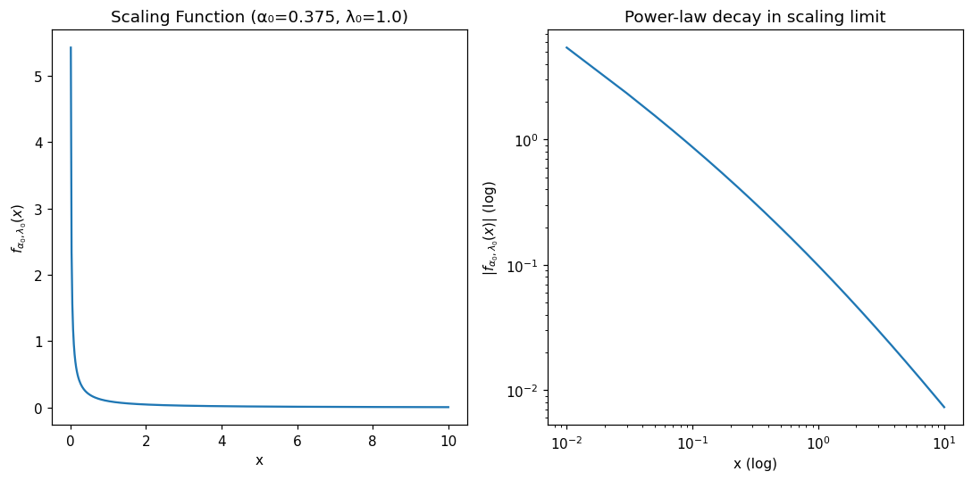
\[\begin{split} E_{\alpha,\beta}(z) \sim \begin{cases} \frac{1}{\alpha} z^{(1-\beta)/\alpha} \exp\!\left(z^{1/\alpha}\right) & z \to +\infty \\[6pt] -\sum_{k=1}^{p} \frac{z^{-k}}{\Gamma(\beta - \alpha k)} + O(|z|^{-p-1}) & z \to -\infty \end{cases} \end{split}\]

The \(f_{\alpha_0, \lambda_0}\) Function¶

From Theorem 3.1 of Muhle-Karbe et al., the key scaling function:

\[ f_{\alpha_0, \lambda_0}(x) = \lambda_0 \, x^{\alpha_0 - 1} \, E_{\alpha_0, \alpha_0}\!\left(-\lambda_0 \, x^{\alpha_0}\right) \]

This function controls how the Hawkes process’s self-excitation structure manifests in the scaling limit. Its integral satisfies:

\[ \int_0^t f_{\alpha_0, \lambda_0}(s) \, ds = t^{\alpha_0} \, E_{\alpha_0, \alpha_0 + 1}\!\left(-\lambda_0 \, t^{\alpha_0}\right) \]

The function \(f_{\alpha_0, \lambda_0}\) interpolates between:

Short times: \(f(x) \sim \lambda_0 x^{\alpha_0 - 1}\) (power-law singularity)
Long times: \(f(x) \sim x^{-1-\alpha_0}\) (power-law decay like the kernel)

Usage Examples¶

Simulating a Hawkes Process¶

import optimizr
import numpy as np
import matplotlib.pyplot as plt

# Simulate with exponential kernel
events_exp = optimizr.simulate_hawkes(
    baseline=1.0,    # ν = 1.0
    alpha=0.5,       # α = 0.5
    beta=1.0,        # β = 1.0
    t_max=100.0,
    kernel_type="exponential",
    seed=42
)

# Simulate with power-law kernel (H₀ ≈ 0.75)
events_pl = optimizr.simulate_hawkes(
    baseline=0.1,
    alpha=0.35,      # K₀ = 0.35
    beta=0.375,      # α₀ = 0.375 → H₀ = 2 × 0.375 = 0.75
    t_max=100.0,
    kernel_type="power_law",
    seed=42
)

print(f"Exponential kernel: {len(events_exp)} events")
print(f"Power-law kernel: {len(events_pl)} events")

Bivariate Buy/Sell Reaction Flow¶

import optimizr
import numpy as np

# Generate core order flow (Poisson driver)
rng = np.random.default_rng(42)
core_buys = np.sort(rng.uniform(0, 100, 200))
core_sells = np.sort(rng.uniform(0, 100, 180))

# Simulate bivariate Hawkes reaction flow
buy_times, sell_times = optimizr.simulate_bivariate_hawkes(
    core_buy_times=core_buys,
    core_sell_times=core_sells,
    phi1_alpha=0.3,   # Self-excitation (buy→buy, sell→sell)
    phi1_beta=1.0,
    phi2_alpha=0.2,   # Cross-excitation (buy→sell, sell→buy)
    phi2_beta=1.0,
    t_max=100.0,
    seed=42
)

print(f"Reaction buys: {len(buy_times)}, Reaction sells: {len(sell_times)}")
print(f"Net order imbalance: {len(buy_times) - len(sell_times)}")

# Check stability
l1_phi1 = 0.3 / 1.0  # L¹ norm of self-excitation
l1_phi2 = 0.2 / 1.0  # L¹ norm of cross-excitation
spectral_radius = l1_phi1 + l1_phi2
print(f"Spectral radius: {spectral_radius:.2f} ({'stable' if spectral_radius < 1 else 'UNSTABLE'})")

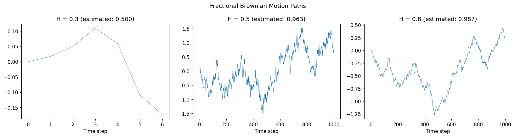
Simulating Fractional Brownian Motion¶

import optimizr
import numpy as np
import matplotlib.pyplot as plt

# Simulate fBM paths with different Hurst exponents
fig, axes = plt.subplots(1, 3, figsize=(15, 4))

for i, h in enumerate([0.3, 0.5, 0.8]):
    path = optimizr.simulate_fbm(hurst=h, n=1000, dt=0.01, seed=42)
    
    # Estimate Hurst exponent from the path
    h_est = optimizr.estimate_hurst(path)
    
    axes[i].plot(path, linewidth=0.5)
    axes[i].set_title(f"H = {h:.1f} (estimated: {h_est:.3f})")
    axes[i].set_xlabel("Time step")

plt.suptitle("Fractional Brownian Motion Paths")
plt.tight_layout()
plt.show()

Generated plot

Mixed fBM for Aggregate Order Flow¶

import optimizr
import numpy as np

# Simulate mixed fBM (BM + fBM with H₀ = 0.75)
path = optimizr.simulate_mixed_fbm(
    a=1.0,       # BM coefficient
    b=1.0,       # fBM coefficient
    hurst=0.75,  # H₀ from unified theory
    n=5000,
    dt=0.01,
    seed=42
)

# Scale-dependent Hurst analysis (identifies mfBM vs pure fBM)
scales = [10, 50, 100, 500, 1000, 2000]
hurst_by_scale = optimizr.scale_dependent_hurst(
    data=path,
    scales=scales
)

print("Scale-Dependent Hurst Exponents:")
print("-" * 35)
for scale, h in sorted(hurst_by_scale.items()):
    print(f"  Scale {scale:>5d}: H = {h:.4f}")

Mittag-Leffler and Scaling Functions¶

import optimizr
import numpy as np
import matplotlib.pyplot as plt

# Verify E_{1,1}(z) = exp(z)
z = 2.0
ml_value = optimizr.mittag_leffler_py(
    alpha=1.0, beta=1.0, z=z
)
print(f"E_{{1,1}}({z}) = {ml_value:.6f}")
print(f"exp({z})     = {np.exp(z):.6f}")

# Plot the scaling function f_{α₀,λ₀}(x)
x = np.linspace(0.01, 10, 500)
alpha_0 = 0.375  # From H₀ = 0.75
lambda_0 = 1.0

f_values = [optimizr.f_alpha_lambda_py(alpha_0, lambda_0, xi) for xi in x]

plt.figure(figsize=(10, 5))
plt.subplot(1, 2, 1)
plt.plot(x, f_values)
plt.xlabel('x')
plt.ylabel(r'$f_{\alpha_0, \lambda_0}(x)$')
plt.title(f'Scaling Function (α₀={alpha_0}, λ₀={lambda_0})')

plt.subplot(1, 2, 2)
plt.loglog(x, np.abs(f_values))
plt.xlabel('x (log)')
plt.ylabel(r'$|f_{\alpha_0, \lambda_0}(x)|$ (log)')
plt.title('Power-law decay in scaling limit')
plt.tight_layout()
plt.show()

Generated plot

Theoretical References¶

Muhle-Karbe, Jusselin & Rosenbaum (2022). A unified approach to the analysis of high-frequency financial markets and limit order books. Annals of Applied Probability.
Jaisson & Rosenbaum (2015). Limit theorems for nearly unstable Hawkes processes. Annals of Applied Probability, 25(2), 600-631.
Bacry, Mastromatteo & Muzy (2015). Hawkes processes in finance. Market Microstructure and Liquidity, 1(01), 1550005.
Mandelbrot & Van Ness (1968). Fractional Brownian motions, fractional noises and applications. SIAM Review, 10(4), 422-437.
Gatheral, Jaisson & Rosenbaum (2018). Volatility is rough. Quantitative Finance, 18(6), 933-949.
Ogata (1981). On Lewis’ simulation method for point processes. IEEE Transactions on Information Theory, 27(1), 23-31.
Hosking (1984). Modeling persistence in hydrological time series using fractional differencing. Water Resources Research, 20(12), 1898-1908.