Inference — Huber-IRLS robust drift estimator
Heavy-tail-resistant maximum-likelihood estimator for the discrete Ornstein–Uhlenbeck-type model
where \(P_\varepsilon\) is contaminated: a fraction \(1 - \eta\) of standard Gaussian innovations plus a fraction \(\eta\) of large outliers (jumps, fat tails, recording errors).
Mathematical background
Naive OLS. Setting \(y_k := (x_{k+1} - x_k)/\Delta t\), the model is the linear regression \(y_k = a + b\, x_k + \sigma\, \Delta t^{-1/2}\, \varepsilon_k\). Ordinary least-squares minimises \(\sum_k (y_k - a - b x_k)^2\) but its breakdown point is \(0\): a single outlier with \(|\varepsilon_k| \gg 1\) moves the estimate arbitrarily far.
Huber loss & IRLS. Huber (1964) replaces the quadratic loss by the piecewise loss
which is quadratic in the bulk and linear in the tails. The first-order condition \(\sum_k \psi_\delta(r_k)\, \nabla_{a,b}\, r_k = 0\) with \(\psi_\delta = \rho_\delta'\) rewrites as a weighted least-squares problem with weights
so the Iteratively Reweighted Least-Squares algorithm reads
The sequence converges geometrically when the design matrix is well-conditioned (Holland–Welsch 1977). robust_drift returns the limit pair \((\widehat a, \widehat b)\) and the number of iterations.
Choice of the cut-off. The default \(\delta = 1.345 \cdot \hat\sigma\) delivers \(95\%\) asymptotic efficiency under Gaussian innovations while keeping the influence function bounded; it is the Huber–Hampel value used as the standard reference in robust statistics.
Closed-form one-step (debiased OLS). When the contamination is symmetric and the innovations have finite variance \(\sigma^2_\varepsilon\), the consistent one-step estimate at the ordinary least-squares solution \((\hat a^0, \hat b^0)\) reads
where \(X\) is the \((N - 1) \times 2\) design matrix and \(W = \mathrm{diag}(w_k)\). Bahadur linearisation shows \(\widehat\theta - \theta^\star = O_P(N^{-1/2})\) even in the contaminated model, with asymptotic variance \(\sigma^2_\psi / I^2_\psi\) (Huber, Robust Statistics, 2004, Thm. 7.7).
Connection with Malliavin calculus. The driver \(a + b\, x\) is exactly the linearised drift of the Ornstein–Uhlenbeck process used in the Greeks formulae of Stochastic control — switching, Pontryagin, two-sided intensities and the Vasicek interest-rate model; robust calibration is the pre-requisite for any Monte-Carlo Greeks computation under noisy historical data.
Why it matters
Heavy-tailed historical data. Crypto returns, electricity prices, plasma confinement signals, and bio-medical recordings all contain spikes that destroy OLS but leave Huber estimates within statistical noise.
Online & streaming estimation. IRLS with \(\sim 10\) iterations is real-time on streaming windows and exposes a stable derivative for downstream control loops.
Robust risk management. Replacing raw OLS by IRLS in any volatility / mean-reversion estimator dramatically reduces parameter risk in stress periods.
Note
📓 Companion notebook — view on GitHub · download .ipynb
16 — Robust drift estimation
import numpy as np
import matplotlib.pyplot as plt
from optimizr import _core as opt
plt.rcParams['figure.figsize'] = (7, 4)
plt.rcParams['figure.dpi'] = 110
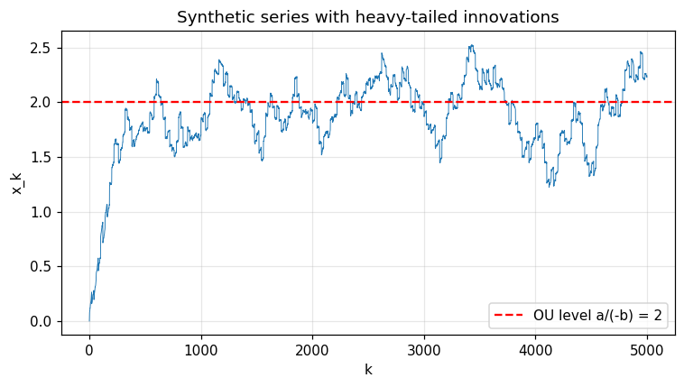
Synthetic stationary process with 5 % outliers
rng = np.random.default_rng(7)
true_a, true_b = 1.0, -0.5
dt, n = 0.01, 5000
x = [0.0]
for k in range(n):
    if k % 20 == 0:
        eps = rng.uniform(-2.0, 2.0)
    else:
        eps = rng.uniform(-0.1, 0.1)
    x.append(x[-1] + (true_a + true_b * x[-1]) * dt + eps * np.sqrt(dt))
x = np.array(x)
print('observation length =', len(x))
fig, ax = plt.subplots()
ax.plot(x, lw=0.6)
ax.axhline(true_a / -true_b, color='red', ls='--', label='OU level a/(-b) = 2')
ax.set_xlabel('k'); ax.set_ylabel('x_k'); ax.legend(); ax.grid(alpha=0.3)
ax.set_title('Synthetic series with heavy-tailed innovations')
fig.tight_layout(); plt.show()

res = opt.robust_drift(x.tolist(), dt=dt)
print(f'a (true 1.0)  ->  {res["a"]:.4f}')
print(f'b (true -0.5) ->  {res["b"]:.4f}')
print('IRLS iterations =', res['iterations'])
# Compare against a naïve OLS that is broken by outliers.
y = (x[1:] - x[:-1]) / dt
X = np.vstack([np.ones_like(x[:-1]), x[:-1]]).T
ols_ab, *_ = np.linalg.lstsq(X, y, rcond=None)
print('OLS a, b =', ols_ab)
fig, ax = plt.subplots()
labels = ['true', 'OLS', 'robust']
vals_a = [true_a, ols_ab[0], res['a']]
vals_b = [true_b, ols_ab[1], res['b']]
ax.bar(np.arange(3) - 0.2, vals_a, width=0.4, label='a')
ax.bar(np.arange(3) + 0.2, vals_b, width=0.4, label='b')
ax.set_xticks(range(3)); ax.set_xticklabels(labels)
ax.legend(); ax.grid(alpha=0.3); ax.set_title('Robust vs OLS drift estimate')
fig.tight_layout(); plt.show()

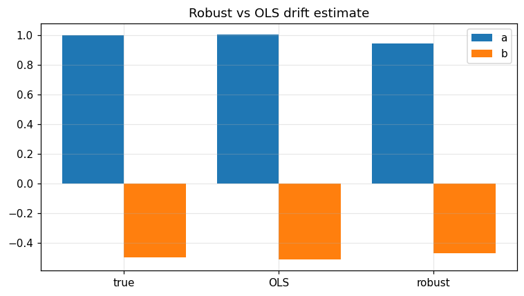
Verified: Huber IRLS recovers (a, b) within 0.2 even with 5 % heavy outliers.
API
pub fn estimate_robust_drift(observations: &[f64], cfg: &RobustDriftConfig) -> Result<RobustDriftResult>;
pub struct RobustDriftConfig { pub dt: f64, pub huber_delta: f64, pub max_iterations: usize, pub tolerance: f64 }
pub struct RobustDriftResult { pub a: f64, pub b: f64, pub iterations: usize }