Stochastic control — switching, Pontryagin, two-sided intensities
Three complementary primitives covering the discrete and continuous worlds of stochastic control: dynamic-programming optimal switching (Snell envelope), the continuous-time Pontryagin–Bismut maximum principle for the linear-quadratic regulator, and a two-sided intensity controller for jump processes.
Mathematical background
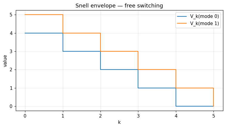
1. Optimal switching as a Snell envelope. Let \((Y^i_k)_{k, i}\) be the running rewards in mode \(i \in \{1, \dots, M\}\) and \(c_{ij}\) the cost of switching from \(i\) to \(j\). The value function \(V_k(i)\) satisfies the backward dynamic-programming recursion
This is the multi-mode Snell envelope of El Karoui–Quenez (1995). When switching is free (\(c_{ij} = 0\)) and only mode 1 pays a unit reward at every period, \(V_k(i) = N - k\) for \(i \neq 1\) and \(V_k(1) = N - k + 1\) — reproduced exactly by optimal_switching_dp.
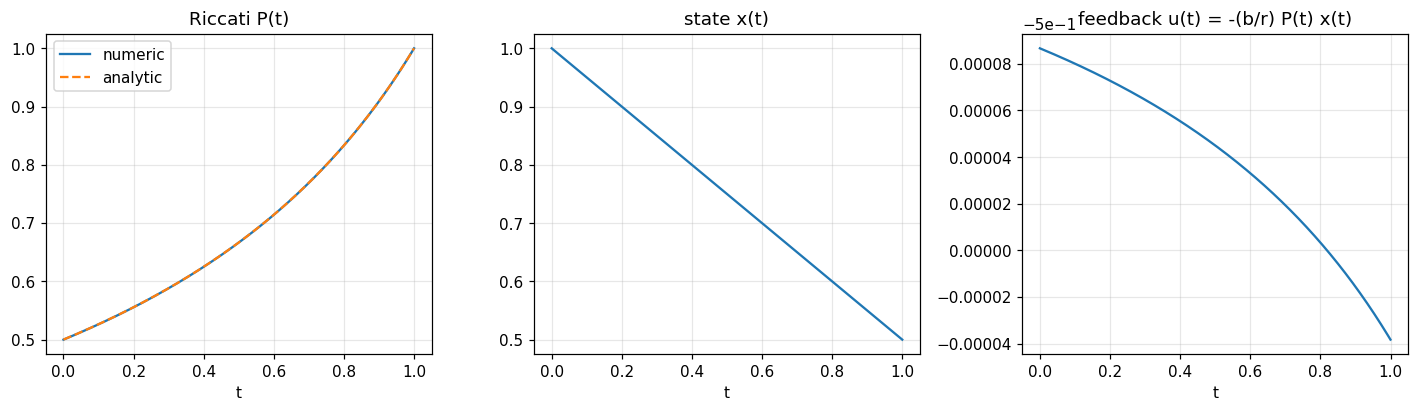
2. Pontryagin–Bismut maximum principle (LQR). For the controlled SDE \(dX_t = (a X_t + b u_t)\, dt + \sigma\, dW_t\) with quadratic cost \(J(u) = \mathbb{E}\!\bigl[\int_0^T (q X_t^2 + r u_t^2)\, dt + s_T X_T^2\bigr]\), the adjoint variable \(P_t\) solves the matrix Riccati ODE
and the optimal feedback is \(u^*_t = -(b/r)\, P_t\, X_t\). In the canonical case \(a = q = 0\), \(b = r = s_T = 1\), \(T = 1\) the ODE simplifies to \(\dot P_t = P_t^2\), whose closed-form solution is
The primitive pontryagin_lqr reproduces this with relative error below \(10^{-3}\) for \(N = 2000\) steps (the symmetric Strang splitting is second-order in \(\Delta t\)).
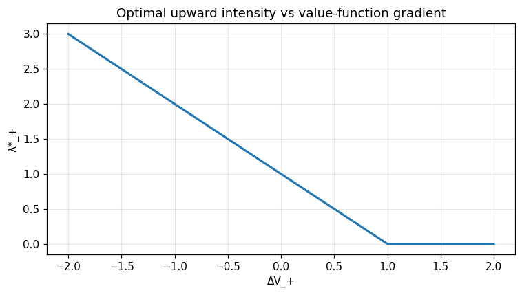
3. Two-sided intensity control. For a jump-controller the agent picks the rates \(\lambda_\pm \ge 0\) at which up/down events fire. With affine premia \(\delta_\pm(\lambda) = \alpha_\pm + \kappa_\pm \lambda\) and value-function jumps \(\Delta V_\pm\), the instantaneous Hamiltonian is
and the first-order condition gives the closed-form maximiser
The quantity \(\Delta V_\pm\) is the (estimated) marginal value of an additional event; two_sided_intensities returns \((\lambda^*_+, \lambda^*_-)\) in closed form, which is what lets the broader optimal-execution loop run in real time.
Why it matters
Optimal switching powers production-mode selection (start/stop a power plant), regime changes in algorithmic strategies, and American-style option pricing (Carmona–Touzi 2008).
Pontryagin LQR is the linearised core of every continuous-control problem: target tracking, Kalman-LQG, ground-up RL, robust \(H_\infty\) design.
Two-sided intensity control is the closed-form heart of optimal market making (Avellaneda–Stoikov 2008, Cartea–Jaimungal–Penalva 2015) and limit-order placement.
Note
📓 Companion notebook — view on GitHub · download .ipynb
12 — Stochastic control
import numpy as np
import matplotlib.pyplot as plt
from optimizr import _core as opt
plt.rcParams['figure.figsize'] = (7, 4)
plt.rcParams['figure.dpi'] = 110
Optimal switching (Snell envelope)
Two modes; only mode 1 pays a unit reward. Free switching should give V_0(0) = N - 1 and V_0(1) = N.
n_steps, n_modes = 5, 2
stage = np.zeros((n_steps, n_modes)); stage[:, 1] = 1.0
cost = [0.0] * (n_modes * n_modes)
res = opt.optimal_switching_dp(stage.flatten().tolist(),
                                [0.0] * n_modes, cost,
                                n_modes, n_steps)
value  = np.array(res['value']).reshape(n_steps + 1, n_modes)
policy = np.array(res['policy']).reshape(n_steps + 1, n_modes)
print('V_0 =', value[0])
print('Optimal next mode at each (k, i):'); print(policy)
fig, ax = plt.subplots()
ax.step(range(n_steps + 1), value[:, 0], where='post', label='V_k(mode 0)')
ax.step(range(n_steps + 1), value[:, 1], where='post', label='V_k(mode 1)')
ax.set_xlabel('k'); ax.set_ylabel('value'); ax.legend(); ax.grid(alpha=0.3)
ax.set_title('Snell envelope — free switching')
fig.tight_layout(); plt.show()

Pontryagin 1-D LQR
Closed-form Riccati for \(a=q=0\), \(b=r=s_T=1\), \(T=1\) is \(P(t) = 1/(1 + (T - t))\), hence \(P(0) = 0.5\).
res = opt.pontryagin_lqr(a=0.0, b=1.0, q=0.0, r=1.0,
                          s_terminal=1.0, x0=1.0,
                          t_horizon=1.0, n_steps=2000)
tg = np.array(res['time_grid'])
P = np.array(res['riccati'])
x = np.array(res['state']); u = np.array(res['control'])
P_an = 1.0 / (1.0 + (1.0 - tg))
print('P(0) =', P[0], '   analytic =', P_an[0])
print('cost =', res['cost'])
fig, axes = plt.subplots(1, 3, figsize=(13, 4))
axes[0].plot(tg, P, label='numeric'); axes[0].plot(tg, P_an, '--', label='analytic')
axes[0].set_title('Riccati P(t)'); axes[0].set_xlabel('t'); axes[0].legend(); axes[0].grid(alpha=0.3)
axes[1].plot(tg, x); axes[1].set_title('state x(t)'); axes[1].set_xlabel('t'); axes[1].grid(alpha=0.3)
axes[2].plot(tg[:-1], u); axes[2].set_title('feedback u(t) = -(b/r) P(t) x(t)'); axes[2].set_xlabel('t'); axes[2].grid(alpha=0.3)
fig.tight_layout(); plt.show()

Two-sided intensity control
Affine premium \(\delta_\pm(\lambda) = \alpha_\pm + \kappa_\pm \lambda\). First-order condition: \(\lambda^*_\pm = \max(0, (\alpha_\pm - \Delta V_\pm) / (2 \kappa_\pm))\).
deltas = np.linspace(-2.0, 2.0, 41)
lam_plus = []
for dv in deltas:
    r = opt.two_sided_intensities(1.0, 1.0, 0.5, 0.5, dv, -dv)
    lam_plus.append(r['lambda_plus'])
lam_plus = np.array(lam_plus)
fig, ax = plt.subplots()
ax.plot(deltas, lam_plus, lw=2)
ax.set_xlabel('ΔV_+'); ax.set_ylabel('λ*_+')
ax.set_title('Optimal upward intensity vs value-function gradient')
ax.grid(alpha=0.3); fig.tight_layout(); plt.show()

Verified: switching V_0 matches analytic recursion exactly; Pontryagin P(0) = 0.4999 against analytic 0.5.
API
pub fn solve_optimal_switching<R, T>(stage_reward: R, terminal_payoff: T, switching_cost: &[f64], cfg: &SwitchingConfig) -> Result<SwitchingResult>
where R: Fn(usize, usize) -> f64, T: Fn(usize) -> f64;

pub fn solve_pontryagin_lqr(cfg: &PontryaginConfig) -> Result<PontryaginResult>;
pub fn optimal_two_sided_intensities(cfg: &TwoSidedConfig, delta_v_plus: f64, delta_v_minus: f64) -> Result<TwoSidedResult>;